This book is in Open Review. I want your feedback to make the book better for you and other readers. To add your annotation, select some text and then click the on the pop-up menu. To see the annotations of others, click the in the upper right hand corner of the page

Chapter 11 Introduction to Bayesian statistics

Learning objectives

Understand differences in how probability is defined in frequentest and Bayesian statistics.
Understand how to estimate parameters and their uncertainty using Bayesian methods.
Compare Bayesian and frequentest inference, starting with a simple problem where we can solve for the Bayesian posterior distribution analytically.

As an aside, you may be surprised to learn that there are multiple ways to define probability. In fact, there are many, many more ways than two; philosophers and mathematicians have long debated the definition and meaning of probability (for an interesting discussion, see: Lyon, 2010).

11.1 R packages

We begin by loading a few packages upfront:

library(kableExtra) # for tables
options(kableExtra.html.bsTable = T)
library(tidyverse) # for data wrangling
library(knitr) # for changing options when knitting
library(ggplot2) # for plotting

In addition, we will use functions from the rgl package (Murdoch & Adler, 2021) for creating a 3-D plot that can be interacted with in the html version of the book.

11.2 Review of frequentist statistics

In frequentist statistics, we define probability in terms of the relative frequency of some event across an infinite sequence of random, repeatable experiments or random trials. This definition of probability is central to key concepts in frequentist statistics:

a sampling distribution describes the distribution of parameter estimates across repeated events (where an event is represented by the process of collecting and analyzing data using the same methods each time).
a null distribution is the distribution of parameter estimates across repeated events in the special situation where the null hypothesis is true.
a confidence interval is an interval that should capture the true unknown parameter for a specified proportion of all events (where now, the event also includes calculating the confidence interval from the sample data).
a p-value is the chance of obtaining a sample statistic as extreme (or more extreme than) an observed sample statistic, if the null hypothesis is true. Again, we consider repeated events of collecting data and calculating the same sample statistic under a situation where the null hypothesis is true.

In frequentist statistics,

Parameters are generally assumed to be fixed quantities that are unknown.
Data are random and used to estimate parameters (e.g., using Maximum Likelihood).
Data are used to test hypotheses which are either TRUE or FALSE.

The goal is to make ‘good’ decisions with high probability (across potential repeated experiments).

11.3 Bayesian statistics

Bayesians also aim to make good decisions with a high probability, but as we will see, probability represents something a little different when it comes to assessing uncertainty in estimation and inference. Specifically, for Bayesians, probability refers to one’s belief given observed data and any prior assumptions about unknown parameters. Although some have criticized Bayesian statistics on the grounds that it is subjective, it is important to stress that Bayesian analyses result in informed beliefs (i.e., informed by data), and in most cases, Bayesian and frequentist analyses will result in similar inferences. Furthermore, although prior beliefs can sometimes make a difference, they are less influential with large data sets.

In Bayesian statistics, all parameters are unknown and their uncertainty is represented by probability distributions (prior distributions before any data are collected and posterior distributions after data have been collected and analyzed).

In Bayesian statistics:

Random variables are used to model all sources of uncertainty. Because parameters are uncertain, they will have a distribution!
Data are treated as fixed and inference is performed conditional on the data.
Prior assumptions are combined with a likelihood, leading to a posterior distribution that describes one’s beliefs about parameters and hypotheses, conditional on the observed data.

Whereas a frequentist will tell you that hypotheses are either true or false (with probability = 1), Bayesians are comfortable quantifying P(Hypothesis | data), which will range between 0 to 1. Bayesians report credible intervals (similar to confidence intervals). These constructs are similar, but Bayesians can and will refer to the probability that a parameter is in a confidencet interval, whereas frequentists will insist that the parameter is in the interval or not (i.e., the probability is 0 or 1).

11.4 Comparing frequentist and Bayesian inference for a simple model

Let’s compare Bayesian and frequentist inference using a simple example. Suppose we are interested in estimating the probability, $p$, that a biologist working with the Minnesota Department of Natural Resources (MN DNR) will detect a moose on the landscape when flying above it in a helicopter. We also want to provide an interval that represents our uncertainty in what $p$ is.

From 2004-2007, the MN DNR conducted a series of detection trials using radiocollared moose to estimate $p$. In each trial, they flew systematic transects within a 4.0 km by 4.3 km area centered around the general vicinity of where a radiocollared moose had been located during the previous week (Figure 11.1). They recorded all moose observed within the plot and in cases where they did not locate the radiocollared moose, they went back and located the individual to determine if it was in the plot when they flew. This resulted in 124 trials during which moose were detected in 59 of them (Giudice et al., 2012).

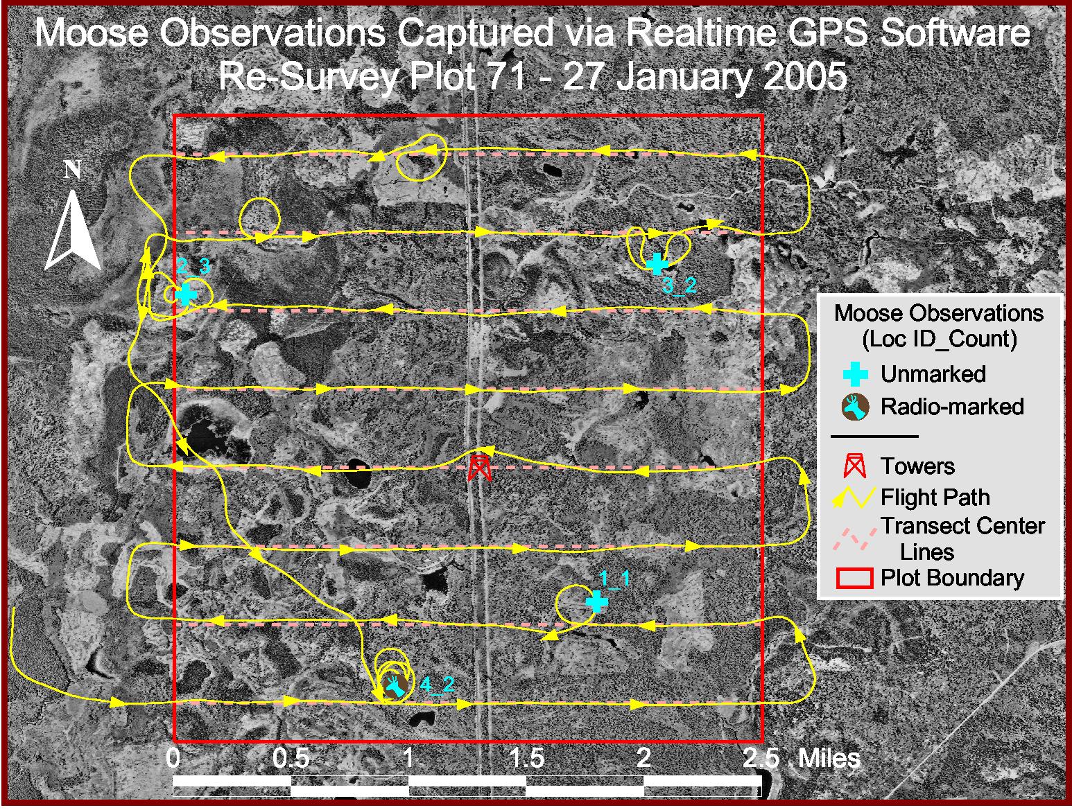
Survey flights used to estimate detection probabilities of radiocollared moose in Minnesota. Flight lines are in yellow. The moose in the lower left was not initially observed. At the end of the flight, this individual was located using the VHF signal on the collar and found to be within the flown plot. Figure created by Robert Wright, Minnesota Department of Natural Resources.

FIGURE 11.1: Survey flights used to estimate detection probabilities of radiocollared moose in Minnesota. Flight lines are in yellow. The moose in the lower left was not initially observed. At the end of the flight, this individual was located using the VHF signal on the collar and found to be within the flown plot. Figure created by Robert Wright, Minnesota Department of Natural Resources.

The probability of detecting a moose will depend on where the moose is located (e.g., the amount of cover that shields the moose from view, termed visual obstruction). We will eventually consider ways to model the probability of detection as a function of the amount of visual obstruction (Chapter 16). For now, however, we will assume that the probability of detection is constant and that all detection trials are mutually independent.

11.4.1 Maximum likelihood

If each trial is independent with constant probability of detection, then we can represent the data-generating process as a Binomial random variable:

\[Y \sim Binomial(124, p),\] with $p$ = probability of a success (i.e., probability of seeing a moose).

The likelihood is thus given by:

$L(p; y) = \frac{n!}{y!(n-y!)}p^{y}(1-p)^{n-y}$

$\Rightarrow \log(L(p; y)) = log(\frac{n!}{y!(n-y!)}) + y\log(p) +(n-y)\log(1-p)$

To use Maximum Likelihood, we consider the likelihood as a function of $p$ and choose the value of $p$ that makes the data as likely as possible. We can maximize $\log[L(p; y)]$ with respect to $p$ by taking the derivative of $\log(L)$ with respect to $p$, set the resulting expression equal to 0, and then solve for $p$:

$\frac{d \log(L(p; y))}{d p} = \frac{y}{p} - \frac{n-y}{1-p} = 0$

Solving for $p$, we obtain the Maximum Likelihood estimator, which turns out to be the sample proportion:

$\hat{p} = y/n$

We could calculate the variance directly using the result that: $Var(ay) = a^2Var(y) \Rightarrow Var(\hat{p}) = Var(y/n) = Var(y)/n^2 = p(1-p)/n$

Alternatively, we could use the asymptotic results from the section on maximum likelihood (Section 10.6) to derive an expression for $var(\hat{p})$. If we were to take second derivatives of $\log(L(p; y))$ with respect to $p$, we would find that:

$I(p) = E\left(-\frac{d^2 \log L(p; n, y)}{dp^2}\right) = \frac{n}{p(1-p)}$. Thus, $var(\hat{p}) = I^{-1}(p) = \frac{p(1-p)}{n}$ (i.e., we end up at the same place as before!).

When our sample size, $n$, is large, we can form a 95% CI using:

\[\hat{p} \pm 1.96\sqrt{\frac{\hat{p}(1-\hat{p})}{n}}.\]

Think-Pair-Share: Where does this expression come from?

In the section on maximum likelihood estimators (Section 10.6), we learned that for large $n$, the sampling distribution of $\hat{p}$ will be Normal, with: $\hat{p} \sim N(p, I^{-1}(p))$, and we just showed that $I^{-1}(p)= \frac{p(1-p)}{n}$. Further:

\[\begin{gather} \hat{p} \sim N\left(p, \frac{p(1-p)}{n}\right) \implies \frac{\hat{p}-p}{\sqrt{\frac{p(1-p)}{n}}} \sim N(0, 1) \\ \implies P(-1.96 \le \frac{\hat{p}-p}{\sqrt{var(\hat{p})}} \le 1.96) = 0.95\\ \implies P\left(\hat{p}-1.96\sqrt{\frac{p(1-p)}{n}} < p < \hat{p}+1.96\sqrt{\frac{p(1-p)}{n}}\right) = 0.95 \end{gather}\]

Lastly, we approximate $\sqrt{\frac{p(1-p)}{n}}$ with $\sqrt{\frac{\hat{p}(1-\hat{p})}{n}}$, giving us the large sample confidence interval you may have seen from an introductory statistics course.

Let’s calculate the large sample, Normal-based confidence interval in R for our moose data:

# Estimate and SE
y <- 54
n <- 124
(p.hat <- y/n)

## [1] 0.4354839

(se.p.hat <- sqrt(p.hat*(1 - p.hat)/124))

## [1] 0.04452597

# Confidence Interval
round(rep(p.hat, 2)+ c(-1.96, 1.96)*se.p.hat, 2)

## [1] 0.35 0.52

Thus, our 95% confidence interval for $p$ is given by $(0.39, 0.56)$.

11.4.2 Aside: how well do these frequentist intervals work

The above confidence interval is based on a large-sample Normal approximation for maximum likelihood estimators. You may have learned in an introductory statistics class that these intervals work well only when $np \ge 10$ and $n(1-p) \ge 10$. Thus, these intervals may not work well with small sample sizes, particularly when $p$ is close to 0 or 1.

We can use simulation to explore how well these intervals perform. Specifically, we will:

Simulate 10,000 binomial random variables using: x <- rbinom(10,000, size = n, p) with a range of values for p and n.
Generate 10,000 estimates of $p$ for each combination of $n$ and $p$, $\hat{p}$ = (x/n).
Generate 10,000 95% CIs for $p$.
Determine how many of these CIs include the true $p$ used to generate the data.

# Create empty object to collect data
simulCIs = data.frame()
# Loop over values of p and n
for (n in seq(5, 200, 1))  {   
    for (p in seq(.05, .95, .05)) { 
      # Simulate "moose detections" (i.e. how many moose you see in the n trials)
      ys <- rbinom(10000, size = n, prob = p)
      p.hats <- ys/n
      se.p.hats <- sqrt(p.hats*(1-p.hats)/n)

      # Calculate 95% confidence intervals
      up.CIs <- p.hats+1.96*se.p.hats 
      low.CIs <- p.hats-1.96*se.p.hats
      
      # Determine the percentage of confidence intervals that contain p
      perc.in.CI <- sum(I(low.CIs < p & up.CIs > p))/10000 

      # Save n, p, and % of CI containing p into the dataframe
      simulCIs <- rbind(simulCIs,c(n,p,perc.in.CI)) 
    }
  }
  #name the columns in the simulation data
  names(simulCIs) <- c("n", "p", "perc.in.CI")

We will use the plot3d function in the rgl library (Murdoch & Adler, 2021) to create a 3-D scatterplot of the results, below (if you are viewing the html version of the book, you should be able to rotate this plot):

FIGURE 11.2: Coverage of large-sample, Normal-based 95 percent confidence intervals for different values of $n$ and $p$ when the data follow a binomial distribution.

We see that the confidence intervals perform well (close to 95% of the intervals contain the true $p$) except when $n$ is really small and $p$ is near 0 or 1.

11.4.3 Bayesian inference for $p$

Let’s see how Bayesian Inference might differ. Here are the steps involved:

Specify a likelihood for the data, $L(y | p)$. Note, in Bayesian formulations, it is common to write the likelihood as a function of the data, $y$, conditional on the set of parameters, $p$. By contrast, in frequentist applications, you may see the likelihood written as a function of the parameters conditional on the data, $L(p | y)$.
Specify a prior distribution for the parameters, $\pi(p)$, reflecting our a priori belief about $p$.
Use Bayes rule (eq. (11.1)) to determine the posterior distribution of $p$ given the data, $p(p | y)$:

\[\begin{equation} p(p | y) = \frac{L(y | p)\pi(p)}{p(y)} = \frac{L(y | p)\pi(p)}{\int L(y | p)\pi(p)dp} \tag{11.1} \end{equation}\]

The posterior distribution, $p(p|y)$, captures our belief about the parameters conditional on the data we observe.

In equation (11.1), $p(y) = \int L(y | p)\pi(p)dp$ is a constant that ensures that the posterior distribution is a proper probability distribution that integrates to 1. $p(y)$ is also referred to as the marginal distribution of $y$ formed by integrating $L(y | p)\pi(p)$ over $p$ (see Section 9.8 for an introduction to marginal distributions). This integral is the continuous version of the total law of probability formula we saw previously in Section 9.2. In most applications, this integral will not have a closed form solution⁵³, so Markov Chain Monte Carlo (MCMC) will be used generate summaries of the posterior distribution (Chapter 12).

Let’s now work through these three steps when analyzing the moose detection data.

Specify a likelihood for the data – we can again use the binomial likelihood:

\[L(y | p) = \frac{124!}{59!(124-59!)} p^{59}(1-p)^{124-59}\]

Specify a prior distribution for $p$. What should we use here? A simple way to narrow our choices is to consider the support for $p$ (the values that $p$ can take on), which in this case is all values between 0 and 1. This leads us naturally to one of two choices:

a uniform distribution on the (0, 1) interval
a beta distribution, since it is the only distribution we have learned about with support on the (0, 1) interval.

The beta distribution has two parameters, $\alpha$ and $\beta$, with probability density function given by:

\[\begin{equation} \pi(p) = \frac{\Gamma(\alpha+\beta)}{\Gamma(\alpha)\Gamma(\beta)} p^{\alpha-1}(1-p)^{\beta-1} \end{equation}\]

Recall from Chapter 9, $\Gamma(z) = \int_0^\infty x^{z-1}e^{-x}dx$ generalizes the factorial function to all complex numbers. For integer values of $z$, $\Gamma(z) = (z-1)! = (z-1)(z-2)\cdots3\times2\times1$.

The beta distribution can take on a number of different shapes depending on the values of $\alpha$ and $\beta$ (see Fig. 11.3), and is equivalent to the uniform distribution when $\alpha = \beta =1$ (you can verify this by plotting the Beta distribution with $\alpha = \beta =1$ in R using curve(dbeta(x, 1, 1), from = 0, to = 1)).

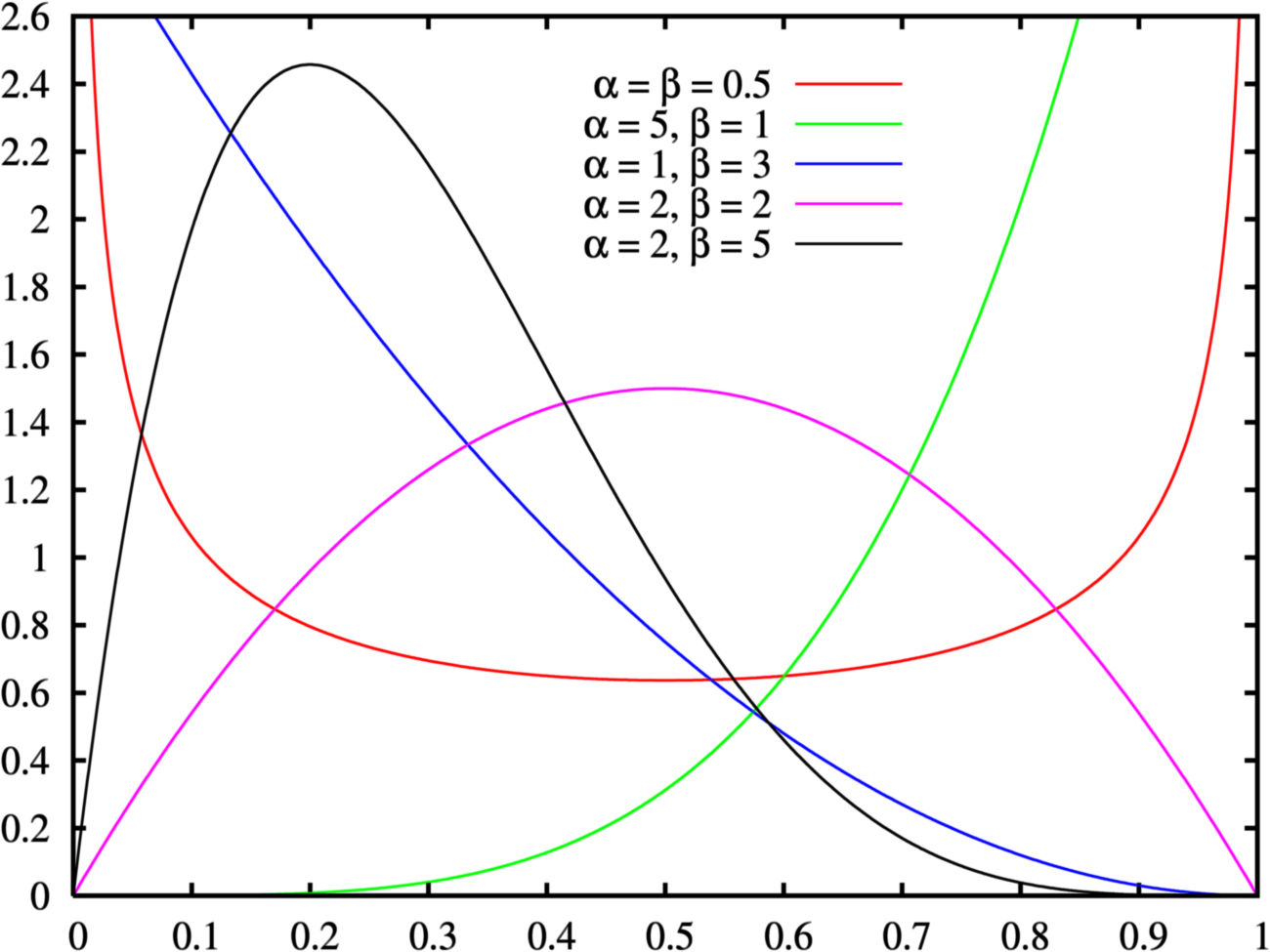
$Probability density functions for beta distributions with different parameters, $\alpha$ and $\beta$.$

FIGURE 11.3: Probability density functions for beta distributions with different parameters, $\alpha$ and $\beta$.

Let’s use a $Beta(1,1) = 1$ (i.e., uniform distribution) for $\pi(p)$, along with the binomial likelihood. We will then use Bayes Theorem to calculate the posterior distribution of $p$, $p(p | y)$.

Rather than write down the full equation for the posterior distribution, including the integral in the denominator, we will use a common trick that works when we have what is called a conjugate prior. A conjugate prior is one that results in a posterior distribution that is from the same family as the prior distribution (in this case, we will see that the posterior distribution is again a beta distribution). To see how this works, we begin by writing down an expression that is proportional to the posterior distribution:

\[\begin{gather} p(p | y) \propto L(y | p)\pi(p) \\ \propto p^{59}(1-p)^{124-59}\cdot 1 \\ \propto p^{60-1}(1-p)^{66-1} \tag{11.2} \end{gather}\]

You may or may not immediately recognize that this expression is proportional to a beta distribution with parameters ($\alpha=60$, $\beta = 66$) (eq. (11.3)):

\[\begin{equation} p(p | y) = \frac{\Gamma(60+66)}{\Gamma(60)\Gamma(66)}p^{60-1}(1-p)^{66-1} \tag{11.3} \end{equation}\]

The constant, $\frac{\Gamma(60+66)}{\Gamma(60)\Gamma(66)}$, ensures that right-hand side of eq. (11.3) integrates to 1 and is therefore a proper probability distribution. This demonstrates a useful trick – if the part of the posterior distribution involving our parameters (i.e., the right-hand side of eq. (11.2)) is proportional to a known distribution, then we can safely assume that this known distribution is in fact our posterior distribution. In the above example, our posterior distribution is a Beta(60, 66) distribution. We can then use this distribution to represent our belief about the likely values for $p$, given the data we observed and our prior assumption that $p$ has a uniform $(0,1)$ distribution.

Let’s use curve to plot the posterior distribution = beta(60, 66):

par(bty = "L", mar=c(2, 4.1, 1, 2.1))
# Plot the Posterior Distribution of theta
plot(curve(dbeta(x, shape1 = 60, shape2 = 66), from = 0, to = 1), 
     type = "l", 
     xlab = expression(theta), 
     ylab = c(expression(p(group("", theta, "|") * y))))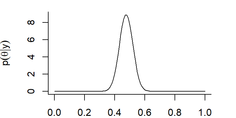

FIGURE 11.4: Posterior distribution for p, the probability of detecting a moose from a helicopter in MN surveys.

We can use this posterior distribution to form a 95% credible interval. To do so, we need to find the endpoints, $x_1$ and $x_2$ such that $P(p \le x_1) = 0.025$ and $P(p \ge x_2) = 0.975$.

Think-Pair-Share: What function in R can we use to calculate these endpoints?

Remember, we can find quantiles of a distribution using q* (in this case, qbeta):

# 95% credible interval
round(qbeta(c(0.025, 0.975), shape1 = 60, shape2 = 66), 2)

[1] 0.39 0.56

We get the exact same endpoints as our frequentist confidence interval! Only now, we are free to say that the probability that $p$ is between 0.39 and 0.56 is 0.95. This statement summarizes our belief about reasonable values of $p$ given the observed data.

11.4.4 Comparing Interpretations: frequentist vs. Bayesian

For this simple problem, we found that our intervals were identical:

frequentist 95% confidence interval for $p$ = (0.39, 0.56)
Bayesian 95% credible interval for $p$ = (0.39, 0.56)

With the Bayesian interval, we can say that the probability that $p$ is in the interval (0.39, 0.56) is 0.95, since this probability represents our belief about $p$ given the data we have collected. By contrast, a frequentist will say that this particular interval either does contain $p$ or it does not contain $p$ (with probability = 1). The parameter itself is a fixed but unknown quantity, and the interval is random (it depends on the observed data). To interpret the frequentist interval in terms of a probability statement, we need to consider creating many such intervals across repeated events (collect data, form interval). We expect that close to 95% of these intervals would contain the fixed and unknown $p$ (see Section 11.4.2). Thus, we say that we are 95% sure that our interval contains the true parameter $p$.

For many readers, the interpretation of the Bayesian interval will seem more natural and this often adds to the appeal of Bayesian methods⁵⁴. Nonetheless, it is still important to consider the performance of Bayesian methods across repeated experiments. For example, we might use simulations to determine if Bayesian 95% credible intervals contain fixed parameters used to simulate data 95% of the time, what statistician Robert Little refers to as calibrated Bayes (Roderick J. Little, 2006).

Often we will find that Bayesian and frequentist methods will lead to a similar conclusions. So, it is helpful to ask, why or when should you prefer to use Bayesian methods? Dorazio (2016) suggests Bayesian inference is most useful in the case of:

Hierarchical models of data that “link a submodel of sampling processes with a submodel of ecological processes.”
Inference for latent (i.e., unobserved) state variables
Missing data problems
Intractable likelihood functions
Complex models of different sources and types of data (with shared parameters); this is currently a hot topic in ecology where integrated population models (Schaub & Kéry, 2021) and integrated species distribution models (Isaac et al., 2020) are frequently used to combine several sources of data when estimating demographic parameters and species distributions, respectively.

In addition, some of you may prefer Bayesian methods in general because:

It is relatively easy to characterize uncertainty for functions of model parameters (no need for the bootstrap or delta method).
The interpretation of credible intervals is appealing.
Bayesian statistics is philosophically appealing since all inferences come from the posterior distribution. There is no need for separate theories for estimation, hypothesis testing, multiple comparisons, etc.

On the other hand, some concerns that arise when using Bayesian statistics include:

With small samples, priors can make a big difference, and therefore, Bayesian methods can be criticized from a standpoint of perceived subjectivity. Furthermore, there are situations where even “vague” priors can end up having a significant influence on the results of an analysis (e.g., Subhash R. Lele, 2020.).
MCMC methods for estimating parameters can be computationally demanding and difficult to implement reliably (though software like JAGS (Plummer et al., 2003) and STAN (Carpenter et al., 2017) help).

These days, many applied statisticians (including me) will use a combination of Bayesian and frequentist methods. Yet, this has not always been the case, and there are still some statistical ecologists that feel strongly that Bayesian methods should not be generally adopted (see e.g., Subhash R. Lele & Dennis, 2009). For example, consider the quote from Dennis (1996) (p. 1095-1103), below:

Ecologists should be aware that Bayesian methods constitute a radically different way of doing science. Bayesian statistics is not just another tool to be added into ecologists’ repertoire of statistical methods. Instead, Bayesians categorically reject various tenets of statistics and the scientific method that are currently widely accepted in ecology and other sciences. The Bayesian approach has split the statistics world into warring factions (ecologists’ “density independence” vs “density dependence” debates of the 1950s pale by comparison), and it is fair to say that the Bayesian approach is growing rapidly in influence

References

Carpenter, B., Gelman, A., Hoffman, M. D., Lee, D., Goodrich, B., Betancourt, M., … Riddell, A. (2017). Stan: A probabilistic programming language. Journal of Statistical Software, 76(1).

Dennis, B. (1996). Discussion: Should ecologists become bayesians? Ecological Applications, 6(4), 1095–1103.

Dorazio, R. M. (2016). Bayesian data analysis in population ecology: Motivations, methods, and benefits. Population Ecology, 58(1), 31–44.

Giudice, J. H., Fieberg, J., & Lenarz, M. S. (2012). Spending degrees of freedom in a poor economy: A case study of building a sightability model for moose in northeastern minnesota. The Journal of Wildlife Management, 76(1), 75–87.

Isaac, N. J., Jarzyna, M. A., Keil, P., Dambly, L. I., Boersch-Supan, P. H., Browning, E., et al.others. (2020). Data integration for large-scale models of species distributions. Trends in Ecology & Evolution, 35(1), 56–67.

Lele, Subhash R. (2020). Consequences of lack of parameterization invariance of non-informative bayesian analysis for wildlife management: Survival of san joaquin kit fox and declines in amphibian populations. Frontiers in Ecology and Evolution, 7, 501.

Lele, Subhash R., & Dennis, B. (2009). Bayesian methods for hierarchical models: Are ecologists making a faustian bargain? Ecological Applications, 19(3), 581–584.

Little, Roderick J. (2006). Calibrated bayes: A bayes/frequentist roadmap. The American Statistician, 60(3), 213–223.

Lyon, A. (2010). Philosophy of probability. Philosophies of the Sciences: A Guide, 92–125.

Murdoch, D., & Adler, D. (2021). Rgl: 3D visualization using OpenGL. Retrieved from https://CRAN.R-project.org/package=rgl

Plummer, M. et al. (2003). JAGS: A program for analysis of bayesian graphical models using gibbs sampling. In Proceedings of the 3rd international workshop on distributed statistical computing (Vol. 124, pp. 1–10). Vienna, Austria.

Schaub, M., & Kéry, M. (2021). Integrated population models: Theory and ecological applications with r and JAGS. Academic Press.

It is difficult to give a precise yet easily digested definition for closed form solution. I like the definition given at https://www.statisticshowto.com/closed-form-solution/, which suggests that the solution should only include: 1) a finite number of symbols, only $+ - *$ and $\div$ operators; and basic functions like $\exp()$, $\log()$, cos(), sin(), etc.↩︎
The same can be said for conclusions from hypothesis tests. Contrast these two conclusions: a) If $H_0$ is true, we would get a result as extreme as the data we saw only 3.2% of the time. Since that is smaller than 5%, we would reject $H_0$ at the 5% level. These data provide significant evidence for the alternative hypothesis; b) The odds in favor of $H_0$ against $H_A$ are 1 to 3. This example is pulled from https://www.austincc.edu/mparker/stat/nov04/talk_nov04.pdf.↩︎

Statistics for Ecologists