This book is in Open Review. I want your feedback to make the book better for you and other readers. To add your annotation, select some text and then click the on the pop-up menu. To see the annotations of others, click the in the upper right hand corner of the page

Chapter 15 Regression models for count data

Learning objectives

1. Understand how maximum likelihood is used to fit modern statistical regression models.
2. Be able to fit regression models appropriate for count data in R and JAGS
   • Poisson regression models
   • Quasi-Poisson (R only)
   • Negative Binomial regression.
3. Interpret estimated coefficients and describe their uncertainty using confidence and credible intervals.
4. Use simple tools to assess model fit
   • Residuals (deviance and Pearson)
   • Goodness-of-fit tests.
5. Use deviances and AIC to compare models.
6. Use an offset to model rates and densities, accounting for variable survey effort.
7. Be able to describe statistical models and their assumptions using equations and text and match parameters in these equations to estimates in R output.

15.1 R packages

We begin by loading a few packages upfront:

library(kableExtra) # for tables
options(kableExtra.html.bsTable = T)
library(sjPlot) # for summarizing output
library(modelsummary) # for creating tables with regression output
library(performance) # for checking model assumptions
library(ggeffects) # for partial residual plots
library(ggthemes) # for colorblind pallete
library(car) # for residual plots
library(dplyr) # for data wrangling
library(MASS) # for glm.nb

In addition, we will use data and functions from the following packages:

• Data4Ecologists for the slugs and longnosedace data sets.
• DHARMa (Hartig, 2021) for creating residual plots and testing goodness of fit
• R2Jags (Y.-S. Su & Masanao Yajima, 2021) for running JAGS code
• MCMCvis (Youngflesh, 2018) for summarizing MCMC output

15.2 Introductory examples: Slugs and Fish

15.2.1 Maximum likelihood: revisiting the slug data

Let’s briefly remind ourselves how we can estimate parameters in a generalized linear model using maximum likelihood. Consider again the slug data from Section 10.3.

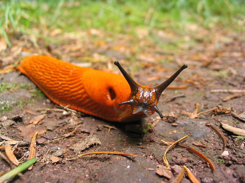
FIGURE 15.1: An orange slug to spice things up (this is not likely the type of slug that was counted). Guillaume Brocker/Gbrocker, CC BY-SA 3.0.

We saw how, using optim, we could fit a model where:

\[Y_i | X_i \sim Poisson(\lambda_i)\]

\[log(\lambda_i) = \beta_0 + \beta_1X_i\]

\[\Rightarrow E[Y_i | X_i] = \mu_i = g^{-1}(\eta) = \exp(\beta_0 + \beta_1X_i)\]

To do this, we relied on the dpois function in R to specify the likelihood. Remember, the general likelihood for the Poisson distribution is given by:

\[L(\beta; y_{1},\ldots, y_{n}, x_{1},\ldots, x_{n}) = \prod_{i=1}^n\frac{\lambda_i^{y_i}\exp(-\lambda_i)}{y_i!}\]

Allowing the \(\lambda_i\) to depend on predictors and regression parameters,\(\lambda_i = exp(\beta_0 + \beta_1x_{i})\), we can write:

\[L(\beta; y_{1},\ldots, y_{n}, x_{1},\ldots, x_{n}) = \prod_{i=1}^n\frac{\exp(\beta_0 + \beta_1x_{i})^{y_i}\exp(-\exp(\beta_0 + \beta_1x_{i}))}{y_i!}\]

And, we can write the log-likelihood as:

\[\log L(\beta; y_{1},\ldots, y_{n}, x_{1},\ldots, x_{n}) = \sum_{i=1}^n \Big(y_i(\beta_0 + \beta_1x_{i})-\exp(\beta_0 + \beta_1x_{i})+ log(y_i!)\Big)\]

We could take derivatives with respect to \(\beta_0\) and \(\beta_1\) and set them equal to 0. However, we would not be able to derive analytical solutions for \(\hat{\beta_0}\) and \(\hat{\beta_1}\). Instead, we (and glm) will use numerical optimization techniques to find the values of \(\beta_0\) and \(\beta_1\) that maximize the log likelihood.

Lets look at how we can use glm to fit this model:

fit.pois <- glm(slugs ~ field, data = slugs, family = poisson())
summary(fit.pois)

Call:
glm(formula = slugs ~ field, family = poisson(), data = slugs)

Coefficients:
             Estimate Std. Error z value Pr(>|z|)    
(Intercept)    0.2429     0.1400   1.735 0.082744 .  
fieldRookery   0.5790     0.1749   3.310 0.000932 ***
---
Signif. codes:  0 '***' 0.001 '**' 0.01 '*' 0.05 '.' 0.1 ' ' 1

(Dispersion parameter for poisson family taken to be 1)

    Null deviance: 224.86  on 79  degrees of freedom
Residual deviance: 213.44  on 78  degrees of freedom
AIC: 346.26

Number of Fisher Scoring iterations: 6

Note, by default, R will use a log link when modeling data using the Poisson distribution. We could, however, use other links by specifying the link argument to the family function as below (for the identity link):

fit.pois <- glm(slugs ~ field, data = slugs, family = poisson(link = "identity"))
summary(fit.pois)

Call:
glm(formula = slugs ~ field, family = poisson(link = "identity"), 
    data = slugs)

Coefficients:
             Estimate Std. Error z value Pr(>|z|)    
(Intercept)    1.2750     0.1785   7.141 9.24e-13 ***
fieldRookery   1.0000     0.2979   3.357 0.000789 ***
---
Signif. codes:  0 '***' 0.001 '**' 0.01 '*' 0.05 '.' 0.1 ' ' 1

(Dispersion parameter for poisson family taken to be 1)

    Null deviance: 224.86  on 79  degrees of freedom
Residual deviance: 213.44  on 78  degrees of freedom
AIC: 346.26

Number of Fisher Scoring iterations: 3

Also, note that by default, R uses effects coding (recall Section 3.7.1). We could, instead, use means coding as follows:

fit.pois <- glm(slugs ~ field - 1, data = slugs, family = poisson())
summary(fit.pois)

Call:
glm(formula = slugs ~ field - 1, family = poisson(), data = slugs)

Coefficients:
             Estimate Std. Error z value Pr(>|z|)    
fieldNursery   0.2429     0.1400   1.735   0.0827 .  
fieldRookery   0.8220     0.1048   7.841 4.46e-15 ***
---
Signif. codes:  0 '***' 0.001 '**' 0.01 '*' 0.05 '.' 0.1 ' ' 1

(Dispersion parameter for poisson family taken to be 1)

    Null deviance: 263.82  on 80  degrees of freedom
Residual deviance: 213.44  on 78  degrees of freedom
AIC: 346.26

Number of Fisher Scoring iterations: 6

Think-Pair-Share: See if you can demonstrate the relationships between the different parameterizations of the Poisson model (means and effects coding and using log and identity links).

15.2.2 Modeling the distribution of longnose dace

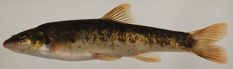
FIGURE 15.2: Picture of a longnose dace. Smithsonian Environmental Research Center, CC BY 2.0.

Let’s consider another count data set collected by the Maryland Biological Stream Survey. The data set includes counts of longnose dace in different sampled areas along with the following predictors:

• stream: name of each sampled stream (i.e., the name associated with each case).
• longnosedace: number of longnose dace (Rhinichthys cataractae) per 75-meter section of stream.
• acreage: area (in acres) drained by the stream.
• do2: the dissolved oxygen (in mg/liter).
• maxdepth: the maximum depth (in cm) of the 75-meter segment of stream.
• no3: nitrate concentration (mg/liter).
• so4: sulfate concentration (mg/liter).
• temp: the water temperature on the sampling date (in degrees C).

We can load the data using:

library(Data4Ecologists)
data("longnosedace")

We begin by fitting a linear model to the data and explore whether the underlying assumptions are reasonable using residual plots constructed using the check_model function in the performance package (Lüdecke et al., 2021) (Figure 15.3).

lmdace <- lm(longnosedace ~ acreage + do2 + maxdepth + no3 + so4 + temp,
             data = longnosedace)
check_model(lmdace, check = c("linearity", "homogeneity", "qq", "normality"))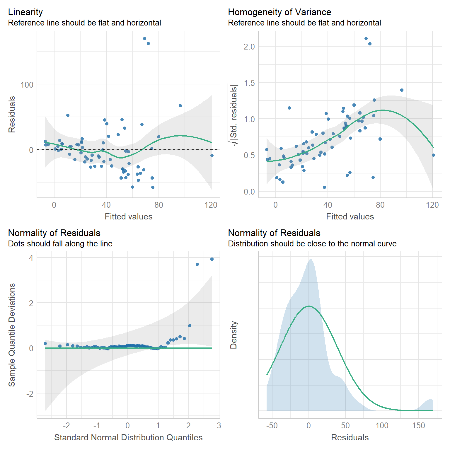

FIGURE 15.3: Residual diagnostic plots for a linear model fit to the longnosedace data.

Examining the plots in the first row, we see that the variance of the residuals increases with fitted values. A reasonable next step might be to consider a Poisson regression model since:

1. Our data are counts and can thus only take on integer values.
2. The variance of the Poisson distribution is equal to the mean (and thus, the variance will increase linearly with the fitted values).

We can fit the Poisson model⁶⁰, below, using the glm function in R:

\[\begin{gather} Dace_i \sim Poisson(\lambda_i) \tag{15.1} \\ \log(\lambda_i) = \beta_0+\beta_1 Acreage_i+ \beta_2 DO2_i + \beta_3 maxdepth_i + \beta_4 NO3_i + \beta_5 SO4_i +\beta_6 temp_i \nonumber \end{gather}\]

glmPdace <- glm(longnosedace ~ acreage + do2 + maxdepth + no3 + so4 + temp, 
              data = longnosedace, family = poisson())
summary(glmPdace)

## 
## Call:
## glm(formula = longnosedace ~ acreage + do2 + maxdepth + no3 + 
##     so4 + temp, family = poisson(), data = longnosedace)
## 
## Coefficients:
##               Estimate Std. Error z value Pr(>|z|)    
## (Intercept) -1.564e+00  2.818e-01  -5.551 2.83e-08 ***
## acreage      3.843e-05  2.079e-06  18.480  < 2e-16 ***
## do2          2.259e-01  2.126e-02  10.626  < 2e-16 ***
## maxdepth     1.155e-02  6.688e-04  17.270  < 2e-16 ***
## no3          1.813e-01  1.068e-02  16.974  < 2e-16 ***
## so4         -6.810e-03  3.622e-03  -1.880   0.0601 .  
## temp         7.854e-02  6.530e-03  12.028  < 2e-16 ***
## ---
## Signif. codes:  0 '***' 0.001 '**' 0.01 '*' 0.05 '.' 0.1 ' ' 1
## 
## (Dispersion parameter for poisson family taken to be 1)
## 
##     Null deviance: 2766.9  on 67  degrees of freedom
## Residual deviance: 1590.0  on 61  degrees of freedom
## AIC: 1936.9
## 
## Number of Fisher Scoring iterations: 5

At this point, we might ask:

• How do we interpret the parameters in the model?
• How can we evaluate the assumptions and fit of the model?
• What tools might we use to select an appropriate set of predictor variables?

15.3 Parameter interpretation

Let’s compare the interpretation of regression coefficients in linear and Poison regression models fit to the dace data (Table 15.1), focusing on the effect of temperature (temp). For the linear regression model, the regression coefficient for temp (equal to 2.75) indicates that the mean number of fish changes by 2.75 as the temperature changes by 1 \(^{\circ}\)C while holding everything else constant. To understand how to interpret the coefficient in the Poisson model, remember that the model is parameterized on the log scale. Thus, a first interpretation that we can offer is that the log mean number of fish changes 0.079 as the temperature changes by 1\(^{\circ}\)C while holding everything else constant. Ideally, however, we would like to interpret the temperature effect on the scale of our observations – i.e., we want to know how temperature relates to the average number of fish in a stream segment, not the log mean.

TABLE 15.1: Parameter estimates (SE) from fitted linear and Poisson regression models.

	Linear regression	Poisson regression
(Intercept)	−127.587 (66.417)	−1.564 (0.282)
acreage	0.002 (0.001)	0.000 (0.000)
do2	6.104 (5.384)	0.226 (0.021)
maxdepth	0.354 (0.178)	0.012 (0.001)
no3	7.713 (2.905)	0.181 (0.011)
so4	−0.009 (0.774)	−0.007 (0.004)
temp	2.748 (1.694)	0.079 (0.007)

It turns out that the Poisson model captures multiplicative effects, which are estimated by exponentiating the regression parameters. To see this, let’s write down our model in terms of the mean, \(E[Y_i|X_i] = \lambda_i\):

\[\lambda_i = \exp(\beta_0+\beta_1 Acreage_i+ \beta_2 DO2_i + \beta_3 maxdepth_i + \beta_4 NO3_i + \beta_5 SO4_i +\beta_6 temp_i)\]

Remembering how exponents work, we can alternatively write:

\[\lambda_i = e^{(\beta_0)}e^{(\beta_1 Acreage_i)}e^{(\beta_2 DO2_i)}e^{(\beta_3 maxdepth_i)} e^{(\beta_4 NO3_i)}e^{(\beta_5 SO4_i)}e^{(\beta_6 temp_i)}\] Now, consider the ratio of means for stream segments that differ only in temp (and by 1 degree C):

\[\frac{\lambda_1}{\lambda_2} = \frac{e^{(\beta_0)}e^{(\beta_1 Acreage_1)}e^{(\beta_2 DO2_1)}e^{(\beta_3 maxdepth_1)} e^{(\beta_4 NO3_1)}e^{(\beta_5 SO4_1)}e^{(\beta_6 (temp_1+1))}}{e^{(\beta_0)}e^{(\beta_1 Acreage_1)}e^{(\beta_2 DO2_1)}e^{(\beta_3 maxdepth_1)} e^{(\beta_4 NO3_1)}e^{(\beta_5 SO4_1)}e^{(\beta_6 temp_1)}}= e^{\beta_6}\] Thus, if we increase temp by 1 unit, while keeping everything else constant, we increase \(\lambda\) by a factor of \(e^{\beta_6}\).

It is common to report rate ratios formed by exponentiating regression parameters as a measure of effect size (Table 15.2)⁶¹. What about confidence intervals for these effect sizes? Again, we can rely on the theory for maximum likelihood estimators from Section 10.6. Specifically, we could use the result that for large samples \(\hat{\beta} \sim N(\beta, I^{-1}(\beta))\) along with delta method (Section 10.8.1) to calculate a confidence interval for \(e^{\beta}\) (for really large samples, it can also be shown that \(e^{\hat{\beta}}\) will also be Normally distributed). It is customary, however, to calculate confidence intervals for \(\beta\) (using the Normal distribution) and then calculate confidence intervals for \(e^{\beta}\) by exponentiating these confidence limits. This is because the sampling distribution for \(\hat{\beta}\) will typically converge to a Normal distribution faster than the sampling distribution for \(\exp(\beta)\) converges to a Normal distribution. Thus, we would calculate the confidence interval for \(\exp(\beta_6)\) associated with temperature using: \(\exp(\hat{\beta}_6 \pm 1.96\widehat{SE}(\hat{\beta}_6))\).

TABLE 15.2: Rate Ratios = \(\exp(\beta)\) (95 percent confidence intervals).

	Poisson regression
(Intercept)	0.209 (0.120, 0.363)
acreage	1.000 (1.000, 1.000)
do2	1.253 (1.202, 1.307)
maxdepth	1.012 (1.010, 1.013)
no3	1.199 (1.174, 1.224)
so4	0.993 (0.986, 1.000)
temp	1.082 (1.068, 1.096)

To calculate these confidence intervals, we need to pull off the variance-covariance matrix for our estimated coefficients using vcov(glmPdace). Taking the square root of the diagonal of this matrix will give us our standard errors.

# store coefficients and their standard errors
beta.hats <- coef(glmPdace)
ses <- sqrt(diag(vcov(glmPdace)))
# Calculate CIs
round(cbind(exp(beta.hats - 1.96*ses), exp(beta.hats + 1.96*ses)), 3)

##              [,1]  [,2]
## (Intercept) 0.120 0.363
## acreage     1.000 1.000
## do2         1.202 1.307
## maxdepth    1.010 1.013
## no3         1.174 1.224
## so4         0.986 1.000
## temp        1.068 1.096

15.4 Evaluating assumptions and fit

15.4.1 Residuals

As with linear models, there are multiple types of residuals that we might consider:

Standard residuals: \(r_i = Y_i - \hat{E}[Y_i | X_i] = Y_i - \hat{Y}_i\). We can access standard residuals using residuals(model, type="response"). If the Poisson distribution is appropriate, we would expect the magnitude of these residuals to increase linearly with \(\lambda_i\) and thus, with \(\hat{E}[Y_i|X_i] = \hat{Y}_i = \hat{\lambda}_i\).

Pearson residuals: \(r_i = \large \frac{Y_i - \hat{E}[Y_i | X_i]}{\sqrt{\widehat{Var}[Y_i | X_i]}}\). We can access Pearson residuals using residuals(model, type="pearson"). If our model is correct, Pearson residuals should have constant variance. You may recall that we considered Pearson residuals when evaluating Generalized Least Squares models in Section 5.

Deviance residuals: \(r_i = sign(y_i-\hat{E}[Y_i | X_i])\sqrt{d_i}\), where \(d_i\) is the contribution of the \(i^{th}\) observation to the residual deviance (as defined in Section 15.4.2) and \(sign = 1\) if \(y_i > \hat{E}[Y_i | X_i]\) and \(-1\) if \(y_i < \hat{E}[Y_i | X_i]\). We can access deviance residuals using residuals(model, type="deviance").

As with linear models, it is common to inspect plots depicting:

• Residuals versus predictors
• Residuals versus fitted values
• Residuals over time or space (to diagnose possible spatial/temporal correlation)

These plots may be useful for identifying whether we should consider allowing for a non-linear relationship between the response and predictor (on the link scale) or if we are missing an important predictor that may be related to temporal or spatial patterning. On the other hand, residual plots for GLMs often exhibit strange patterning due to the discrete nature of the data (e.g., counts can take on only integer values and binary responses have to be either 0 or 1). Thus, it can help to add a smooth curve to the plot to diagnose whether there is a pattern in residuals (e.g., as we increase from small to large fitted values). The residualPlots function in the car package (Fox & Weisberg, 2019) will do this for us (Figure 15.4). It also returns goodness-of-fit tests aimed at detecting whether the relationship between predictor and response is non-linear on the transformed scale (i.e., log in the case of Poisson regression models).

residualPlots(glmPdace)

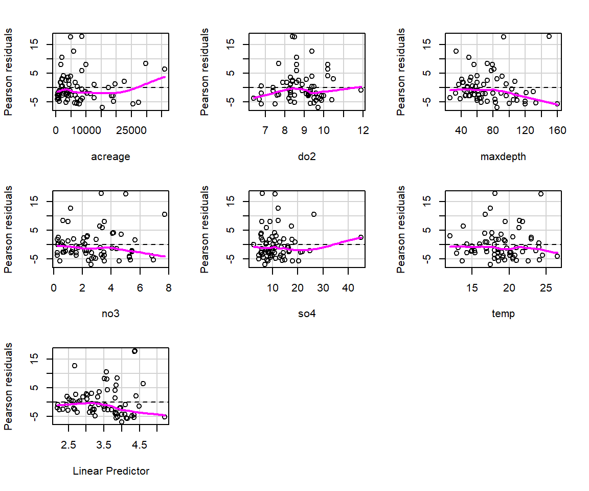
FIGURE 15.4: Plots of residuals versus each predictor and against fitted values using the residualPlots function in the car package (Fox & Weisberg, 2019).

##          Test stat Pr(>|Test stat|)    
## acreage    50.3494        1.287e-12 ***
## do2        40.9062        1.597e-10 ***
## maxdepth   12.8087         0.000345 ***
## no3         0.0670         0.795691    
## so4        22.0158        2.704e-06 ***
## temp        1.2443         0.264652    
## ---
## Signif. codes:  0 '***' 0.001 '**' 0.01 '*' 0.05 '.' 0.1 ' ' 1

The goodness-of-fit tests suggest there are problems with this model, and indeed, my experience has been that the Poisson model rarely provides a good fit to ecological data. We will further consider goodness-of-fit testing in Section 15.4.5.

Another popular alternative for evaluating fit of generalized linear models, including models with random effects (Sections 18 and 19), is to use simulation-based approaches available in the DHARMa package (Hartig, 2021). DHARMa creates simulated residuals that are transformed to lie between 0 and 1 (Figure 15.5) via the following steps:

1. New response data are simulated from the fitted model for each observation (similar to the process we used to conduct the goodness-of-fit test in Section 13.4).

2. For each observation, the cumulative distribution function of the simulated data (associated with that observation’s predictor values) is used to determine a standardized residual under the assumed model. If the observation is smaller than all of its corresponding simulated data points, then the residual will be 0. If it is larger than 50% of the simulated data points, it will have a residual of 0.5. And if it is larger than all of the simulated data points, it will have a residual of 1.

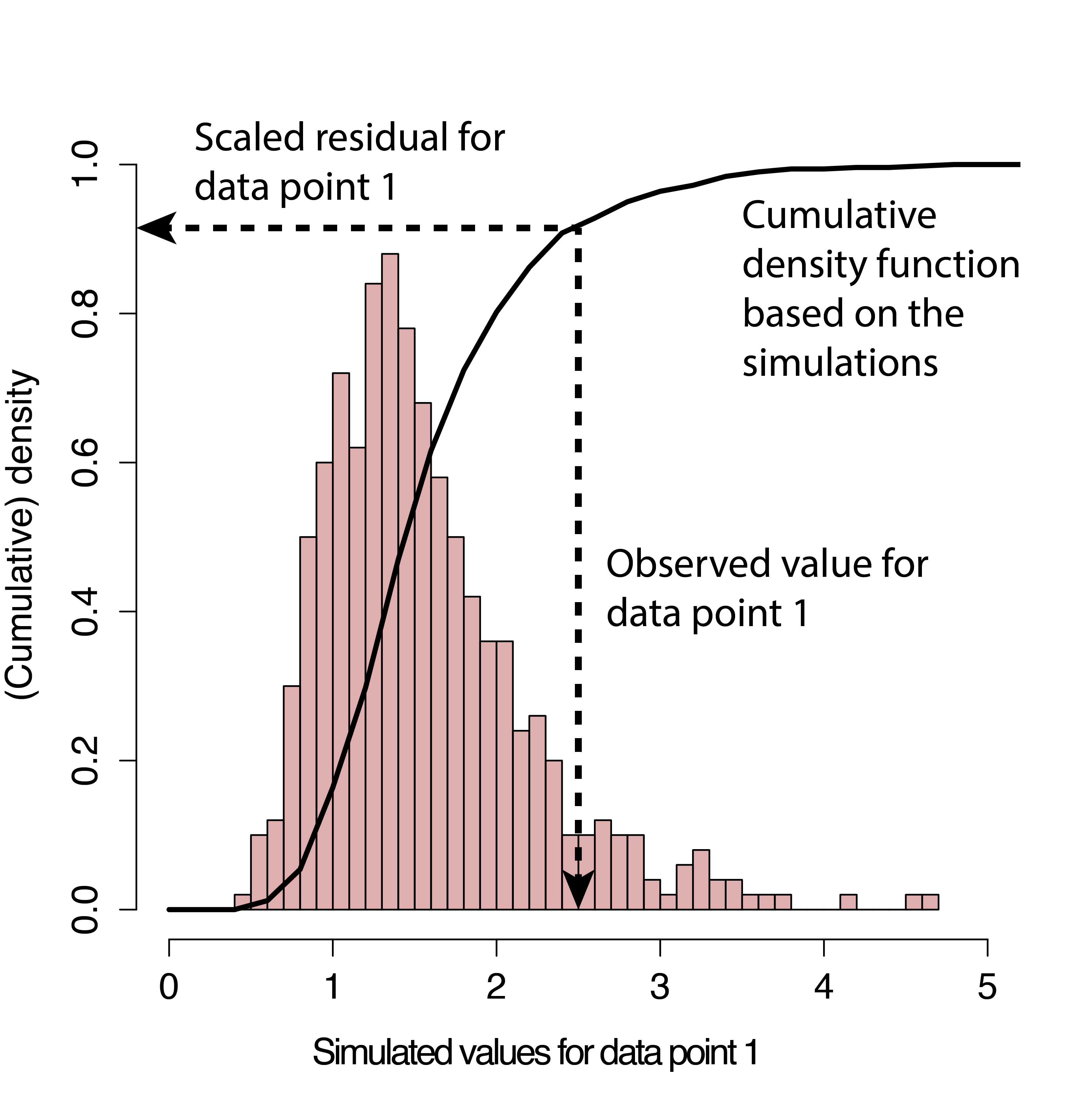
FIGURE 15.5: Simulation-based process for creating standardized residuals via the DHARMa package (Hartig, 2021). Figure is copied from the DHARMa vignette.

If the model is appropriate for the data, then we should expect the distribution of the residuals to be uniform (all values should be equally likely). A nice thing about this approach is that it can work with any type of model (linear model, generalized linear model, etc).

The main workhorse of the DHARMa package is the simulateResiduals function, which implements the algorithm above.

library(DHARMa)
simulateResiduals(glmPdace, plot = TRUE)

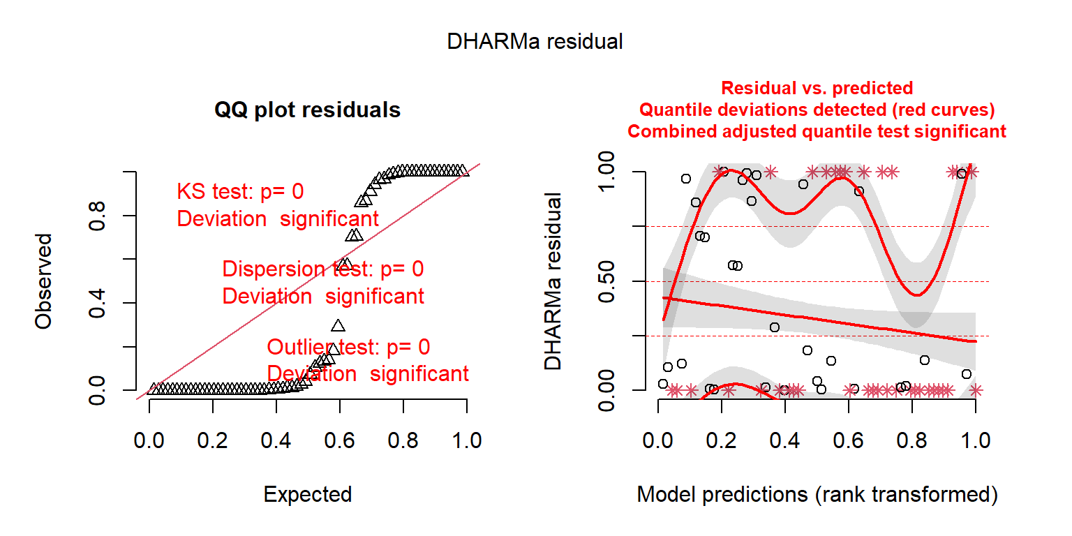
FIGURE 15.6: DHARMa residual plots for the Poisson regression model fit to the longnose Dace data.

## Object of Class DHARMa with simulated residuals based on 250 simulations with refit = FALSE . See ?DHARMa::simulateResiduals for help. 
##  
## Scaled residual values: 0.01291999 0 0.9107332 0.004 0.9422699 0 1 1 0 0 0.139003 0.8586797 0 0.2893398 0 0.9675016 0 0.9996452 0.002739775 0 ...

By adding plot = TRUE, the function also provides us with two plots (Figure 15.6). The first plot on the left is a Quantile-Quantile (QQ) plot for a uniform (0, 1) distribution. If the model is appropriate, the points should fall on the 1-1 line. DHARMa also provides test statistics and p-values associated with tests for whether the distribution is uniform, whether the residuals are overdispersed, and whether their are outliers. In this case, all three tests suggest the model provides a poor fit to the data. The second plot (on the right) is a residuals versus fitted values plot. Observations that fall outside of the range of simulated values are highlighted as outliers (red stars). DHARMa also performs a quantile regression to compare empirical and theoretical 0.25, 0.5 and 0.75 quantiles and provides a p-value for a test of whether these differ from each other.

15.4.2 Aside: Deviance and pseudo-R\(^2\)

Let \(\theta\) be a set of parameters to be estimated by maximum likelihood (in the context of our above example, \(\theta\) is the set of regression coefficients, \(\beta_0\) through \(\beta_6\)). The deviance is a measure of model fit when using maximum likelihood.

The residual deviance, \(D_0\), is given by:

\[D_0= 2(logL(y| \hat{\theta}_s)-logL(y|\hat{\theta}_0)), \mbox{where}\]

• \(logL(\hat{\theta}_s | y)\) = log-likelihood for a “saturated” model (one with a parameter for each observation).
• \(logL(\hat{\theta}_0 | y)\) = log-likelihood for our model of interest evaluated at the maximum likelihood estimates (\(\hat{\theta}_0\)).

The null deviance is the residual deviance for a model that only contains an intercept. It may be helpful to think of the null deviance and residual deviance as maximum likelihood equivalents of total and residual sums of squares, respectively.

There is no \(R^2\) for generalized linear models, but it is not uncommon to see percent deviance explained in regression output and also reported as a (pseudo \(R^2\)) measure (Faraway, 2016):

\[\begin{gather} \text{pseudo }R^2 = 100 \times \frac{\mbox{null deviance - residual deviance}}{\mbox{null deviance}} \tag{15.2} \end{gather}\]

This is easy to calculate from the fitted model:

 1-(glmPdace$deviance/glmPdace$null.deviance)

## [1] 0.4253322

Like \(R^2\) for linear models, the above pseudo-\(R^2\) will range between 0 and 1, with higher values indicating better fit. On the other hand, it should not be interpreted in the same way as the \(R^2\) in a linear model (as the proportion of variance in the response explained by the model), and its values may be considerably lower than users of \(R^2\) in linear models have come to expect (e.g., McFadden, 1977 suggests values of 0.2-0.4 describe excellent fit in the context of logistic regression). Also, note there have been many other pseudo-\(R^2\) measures proposed, and none are without controversy. For more information regarding other measures of pseudo \(R^2\), how to calculate them, and potential considerations when using them, see this FAQ for pseudo-R\(^2\) in the context of logistic regression. In addition, Nakagawa & Schielzeth (2013) reviews several pseudo-\(R^2\) metrics proposed for generalized linear models before proposing new metrics for use with mixed models that are the subject of Chapters 18 and 19. Lastly, we note that the performance package has an r2() function for calculating various \(R^2\) metrics for a variety of models, including generalized linear models and mixed-effect models. It will return a list containing values for what the authors deem to be the “most appropriate” \(R^2\) for a given model type. Below, we apply this function to our Poisson regression model, which returns a value of 1 (which I find to be quite surprising).

r2(glmPdace)

## # R2 for Generalized Linear Regression
##   Nagelkerke's R2: 1.000

If you try other options, you will get very different results. For example, we get a much lower value when using the r2_mcfadden() function.

r2_mcfadden(glmPdace)

## # R2 for Generalized Linear Regression
##        R2: 0.380
##   adj. R2: 0.379

Personally, I do not find all that much value in these different \(R^2\) measures. I would much rather inspect effect plots to get a feel for the amount of unexplained variation (e.g., Figure 15.7). These plots will be explored in more detail in Section 16.6.

sjPlot::plot_grid(plot(ggpredict(glmPdace), add.data = TRUE, one_plot = FALSE))

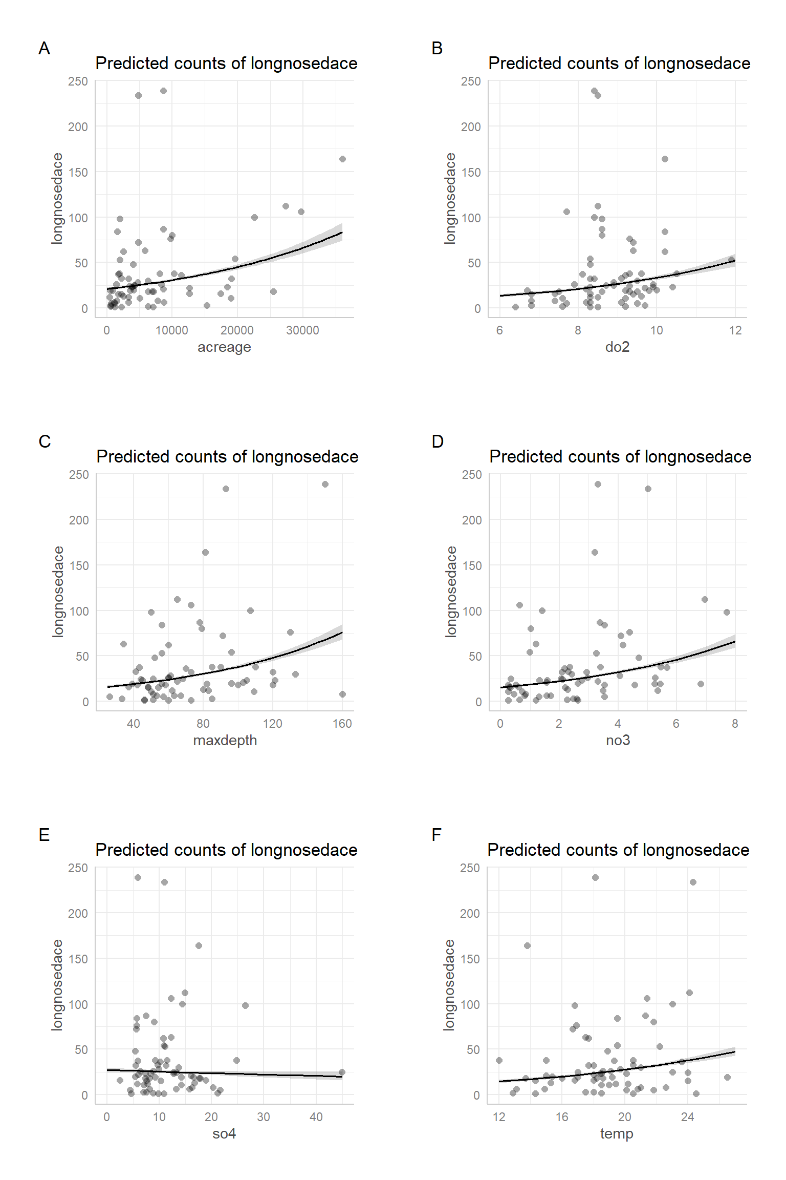
FIGURE 15.7: Partial residual plots for the Poisson regression model fit to the longnose dace data.

15.4.3 Overdispersion: What is it?

The Poisson distribution assumes \(Var(Y_i|X_i) = E(Y_i|X_i)\). When the variance is greater than the mean, we say the data are overdispersed relative to the Poisson distribution. There are many reasons why data may be overdispersed:

• We may have omitted important predictor variables
• Explanatory and response variables may be measured with error
• Our model may be mis-specified (e.g., the relationship between log(\(\lambda\)) and \(X\) may be non-linear)
• Our data set may include one or more large outliers
• Our data may exhibit significant spatial, temporal, within-individual clustering (e.g., as may be the case when we have more than one observation on each sample unit)

Lastly, the response variable may result from a mixture of random processes. In wildlife monitoring data sets, for example, we might consider that:

• One set of environmental variables may determine whether a particular habitat is suitable for a given species, and thus, whether a site is occupied or not.
• A second, possibly overlapping set of variables, may determine the density in suitable habitat.

This situation can lead to data sets with an overabundance of zeros. Zero-inflated models (Section 17) have been developed to accommodate this situation.

15.4.4 Simple tests for overdispersion

Given that the mean and variance are likely to both depend on predictors, \(X\), how should we diagnose possible overdispersion? It is not uncommon to compare the residual deviance \(D_0\) or Pearson’s \(\chi^2\) statistic \(\sum_{i=1}^n \frac{(Y_i-E[Y_i|X_i])^2}{Var[Y_i | X_i]}\) to a \(\chi^2\) distribution with \(n-p\) degrees of freedom to detect overdispersion. The check_overdispersion function in the performance package provides a test based on the Pearson \(\chi^2\) statistic.

check_overdispersion(glmPdace)

## # Overdispersion test
## 
##        dispersion ratio =   29.403
##   Pearson's Chi-Squared = 1793.599
##                 p-value =  < 0.001

## Overdispersion detected.

Yet, the \(\chi^2\) distributional assumption may not be appropriate especially when the number of observations with a given suite of predictors is small (e.g. \(\le 5\)) as will typically be the case when the model contains continuous predictors. Thus, it is usually best to test for overdispersion using (predictive) simulation techniques discussed in Section 15.4.5.

15.4.5 Goodness-of-fit test using predictive simulation

In Section 15.4.1, we saw that the residualPlots function in the car package provided a lack-of-fit test for each predictor in the model. In this section, we will consider a general approach to assessing goodness-of-fit that is analogous to the Bayesian p-value we saw in Section 13.4.

First, it may be helpful to review the different steps involved in any statistical hypothesis test in the context of a goodness-of-fit test:

1. State Null and Alternative hypotheses:

   • \(H_0\): the data are consisten with the assumed Poisson regression model given by eq. (15.1)

   • \(H_A\): the data are not consistent with the assumed model

2. Calculate a test statistic that measures the discrepancy between the data and the null hypothesis.

3. Determine the distribution of the test statistic in step 2, when the null hypothesis is true.

4. Compare the statistic for the observed data [step 2] to the distribution of the statistic when the null hypothesis is true [step 3]. The p-value is the probability that the GOF statistic for the observed data is as or more extreme than GOF statistic for data collected under situations where the null hypothesis is true.

If p-value is small, then we have evidence that the model is not appropriate. If the p-value is not small, then we do not have enough evidence to suggest the model is not appropriate (whew!).

OK, let’s begin by considering how to formulate a goodness-of-fit test for the Poisson model. Like the Bayesian p-value approach, we will want to account for our uncertainty due to having to estimate \(\lambda_i\). Because glm uses maximum likelihood to estimate parameters, we know that the sampling distribution of \(\hat{\beta}\), when \(n\) is large, is given by:

\[\hat{\beta} \sim N(\beta, cov(\hat{\beta})),\]

where \(cov(\hat{\beta})=I^{-1}(\hat{\beta})\), the inverse of the Hessian. For models fit using glm, we can access an estimate of the variance covariance matrix, \(\widehat{cov}(\hat{\beta})\), using vcov(model). Thus, we can account for parameter uncertainty by drawing random parameters from a multivariate normal distribution with mean = \(\hat{\beta}\) and variance/covariance matrix = \(\widehat{cov}(\hat{\beta})\). From these parameter values, we calculate \(\hat{\lambda} = exp(X\hat{\beta})\) for each of our observations.

We also need the ability to simulate new data sets where the null hypothesis is true (in this case, our model is correct). We can do this using the rpois function. Lastly, we will need to calculate a measure of fit for both real and simulated data. There are many possibilities here depending on what sort of lack-of-fit you might want to be able to detect. One possibility is to use the Pearson \(\chi^2\) statistic (e.g., Kéry, 2010, Chapter 13):

\[\chi^2_{n-p} = \sum_{i=1}^n \frac{(Y_i-E[Y_i|X_i])^2}{Var[Y_i | X_i]}\].

The p-value for our test is given by the proportion of samples where \(\chi^2_{sim}\ge \chi^2_{obs}\). If the model is appropriate, “goodness-of-fit” statistics for real and simulated data should be similar. If not, the model should fit the simulated data much better than the real data and our p-value will be small. A small p-value would lead us to reject the null hypothesis that our model is appropriate for the data.

We implement this approach using 10,000 simulated data sets below:

# Number of simulations
  nsims <- 10000

# Set up matrix to hold goodness-of-fit statistics
  gfit.sim <- gfit.obs <- matrix(NA, nsims, 1)
  nobs <- nrow(longnosedace) # number of observations
  
# Extract the estimated coefficients and their asymptotic variance/covariance matrix  
# Use these values to generate nsims new betas  
  beta.hat <- MASS::mvrnorm(nsims, coef(glmPdace), vcov(glmPdace))

# Design matrix for creating new lambda^s    
  xmat <- model.matrix(glmPdace)
  for(i in 1:nsims){
    # Generate lambda^s, note that %*% is used fo rmatrix mulitplication   
    lambda.hat <- exp(xmat%*%beta.hat[i,])
    
    # Generate new simulated values
    new.y <- rpois(nobs, lambda = lambda.hat)
    
    # Calculate Pearson Chi-squared statistics
    gfit.sim[i,] <- sum((new.y-lambda.hat)^2/(lambda.hat))
    gfit.obs[i,] <- sum((longnosedace$longnosedace-lambda.hat)^2/lambda.hat)
  }
  # Calculate and print the p-value
  (GOF.pvalue <- mean(gfit.sim > gfit.obs))

## [1] 0

We see that the p-value is essentially 0, suggesting again that the Poisson model is not a good model for these data. The Pearson \(\chi^2\) statistic was always larger for the observed data than the simulated data.

15.5 Quasi-Poisson model for overdispersed data

What are the consequences of analyzing the data using Poisson regression when the data are overdispersed? If the model for the transformed mean, \(\log(E[Y_i|X_i]) = \beta_0 + \beta_1X_1+\ldots \beta_p X_p\) is appropriate, but the Poisson distribution is not, then our estimates of \(\beta\) may be unbiased but their standard errors may be too small. In addition, p-values for hypothesis tests will also be too small and may lead us to select overly complex models if we use hypothesis tests to select predictors to include in our models.

If we are happy with our model for the transformed mean, \(\log(E[Y_i|X_i]) = \beta_0 + \beta_1X_1+\ldots \beta_p X_p\), we might also consider two relatively simple approaches:

1. We can use a bootstrap to calculate standard errors and confidence intervals (see Chapter 2).
2. We can adjust our standard errors using a variance inflation parameter.

With both approaches, we relax the assumption that \(Y_i|X_i \sim Poisson\). The second approach, however, adds an assumption regarding the variance of \(Y_i|X_i\). In particular, we assume:

• \(E[Y_i|X_i] = \mu_i = e^{\beta_0 + \beta_1X_{1,i} + \ldots + \beta_pX_{p,i}}\)
• \(Var[Y_i|X_i] = \phi\mu_i = \phi e^{\beta_0 + \beta_1X_{1,i} + \ldots + \beta_pX_{p,i}}\)

Although we make assumptions about the mean and variance, we do not specify a probability distribution for the data, and therefore, we are not technically using likelihood-based methods. Rather, this approach has been termed quasi-likelihood (McCullagh & Nelder, 1989)⁶². We can estimate the scale parameter, \(\hat{\phi}\) by either:

• \(\hat{\phi} = \frac{\mbox{Residual deviance}}{(n-p)}\)
• \(\hat{\phi} = \frac{1}{n-p}\sum_{i=1}^n \frac{(Y_i-E[Y_i|X_i])^2}{Var[Y_i | X_i]}\) (this is the approach R takes)

In R, we can fit the quasi-likelihood model as follows:

glmQdace<-glm(longnosedace ~ acreage + do2 + maxdepth + no3 + so4 + temp, 
              data = longnosedace, family = quasipoisson())  
summary(glmQdace)

## 
## Call:
## glm(formula = longnosedace ~ acreage + do2 + maxdepth + no3 + 
##     so4 + temp, family = quasipoisson(), data = longnosedace)
## 
## Coefficients:
##               Estimate Std. Error t value Pr(>|t|)   
## (Intercept) -1.564e+00  1.528e+00  -1.024  0.30999   
## acreage      3.843e-05  1.128e-05   3.408  0.00116 **
## do2          2.259e-01  1.153e-01   1.960  0.05460 . 
## maxdepth     1.155e-02  3.626e-03   3.185  0.00228 **
## no3          1.813e-01  5.792e-02   3.130  0.00268 **
## so4         -6.810e-03  1.964e-02  -0.347  0.73001   
## temp         7.854e-02  3.541e-02   2.218  0.03027 * 
## ---
## Signif. codes:  0 '***' 0.001 '**' 0.01 '*' 0.05 '.' 0.1 ' ' 1
## 
## (Dispersion parameter for quasipoisson family taken to be 29.40332)
## 
##     Null deviance: 2766.9  on 67  degrees of freedom
## Residual deviance: 1590.0  on 61  degrees of freedom
## AIC: NA
## 
## Number of Fisher Scoring iterations: 5

Here, the inflation parameter is estimated to be 29.4. Comparing the estimates and standard errors to our Poisson regression model, we see that \(\hat{\beta}\) is unchanged, but the SEs are all larger by a factor of \(\sqrt{\phi} = \sqrt{29.4}\).

When is it reasonable to use this approach? Zuur et al. (2009) suggest that a quasi-Poisson model may be appropriate when \(\phi > 1.5\), but that other methods should be considered when \(\phi\) is greater than 15 or 20. These other methods might include, Negative Binomial regression (see Section 15.6), zero-inflation models (see Chapter 17), or a Poisson-normal model (see Section 15.8.3).⁶³

15.6 Negative Binomial regression

In my experience, most count data sets collected by ecologists are overdispersed relative to the Poisson distribution. The Negative Binomial distribution offers a useful alternative in these cases. We will consider the following parameterization of the Negative Binomial distribution:

\(Y_i|X_i \sim\) NegBin(\(\mu_i, \theta\)), with \(E[Y_i|X_i] = \mu_i\) and \(var[Y_i|X_i] = \mu_i + \frac{\mu_i^2}{\theta}\)

The Negative Binomial distribution is overdispersed relative to Poisson, with:

\[\frac{Var[Y_i|X_i]}{E[Y_i|X_i]} = 1 + \frac{\mu}{\theta}\]

When \(\theta\) is large, the Negative Binomial model will converge to a Poisson with variance equal to the mean.

We can use the glm.nb function in the MASS library to fit a Negative Binomial Regression model to the dace data. Like when using glm to fit Poisson regression models, the default is to model the log mean as a function of predictors and regression coefficients (eq. (15.3)):

\[\begin{gather} Dace_i \sim \mbox{Negative Binomial}(\mu_i, \theta) \tag{15.3} \nonumber \\ \log(\mu_i) = \beta_0+\beta_1 Acreage_i+ \beta_2 DO2_i + \beta_3 maxdepth_i + \nonumber \\ \beta_4 NO3_i + \beta_5 SO4_i +\beta_6 temp_i \nonumber \end{gather}\]

glmNBdace <- MASS::glm.nb(longnosedace ~ acreage + do2 + maxdepth + no3 + so4 + temp, 
                          data = longnosedace)
summary(glmNBdace)

## 
## Call:
## MASS::glm.nb(formula = longnosedace ~ acreage + do2 + maxdepth + 
##     no3 + so4 + temp, data = longnosedace, init.theta = 1.666933879, 
##     link = log)
## 
## Coefficients:
##               Estimate Std. Error z value Pr(>|z|)    
## (Intercept) -2.946e+00  1.305e+00  -2.256 0.024041 *  
## acreage      4.651e-05  1.300e-05   3.577 0.000347 ***
## do2          3.419e-01  1.050e-01   3.256 0.001130 ** 
## maxdepth     9.538e-03  3.465e-03   2.752 0.005919 ** 
## no3          2.072e-01  5.627e-02   3.683 0.000230 ***
## so4         -2.157e-03  1.517e-02  -0.142 0.886875    
## temp         9.460e-02  3.315e-02   2.854 0.004323 ** 
## ---
## Signif. codes:  0 '***' 0.001 '**' 0.01 '*' 0.05 '.' 0.1 ' ' 1
## 
## (Dispersion parameter for Negative Binomial(1.6669) family taken to be 1)
## 
##     Null deviance: 127.670  on 67  degrees of freedom
## Residual deviance:  73.648  on 61  degrees of freedom
## AIC: 610.18
## 
## Number of Fisher Scoring iterations: 1
## 
## 
##               Theta:  1.667 
##           Std. Err.:  0.289 
## 
##  2 x log-likelihood:  -594.175

The estimate of \(\theta\) = 1.667 suggests the data are overdispsersed relative to the Poisson. If we compare the Poisson and Negative Binomial models using AIC, we find strong evidence in favor of the Negative Binomial model:

AIC(glmPdace, glmNBdace)

##           df       AIC
## glmPdace   7 1936.8602
## glmNBdace  8  610.1754

Think-Pair-Share (Review): How could we use R’s functions for probability distributions to calculate these AIC values?

df.model1 <- 7
df.model2 <- 8
-2*sum(dpois(longnosedace$longnosedace, 
             lambda = predict(glmPdace, type = "resp"), 
             log = TRUE)) + 2 * df.model1

## [1] 1936.86

-2*sum(dnbinom(longnosedace$longnosedace, 
               mu = predict(glmNBdace, type = "resp"), 
               size = glmNBdace$theta, log = TRUE)) + 2 * df.model2

## [1] 610.1754

Let’s use the residualPlot function in the car library to construct a Pearson residual versus fitted value plot for both the Poisson and Negative Binomial regression models (Figure 15.8). Neither plot looks perfect, but the variance seems a little more constant for the Negative Binomial model.

residualPlot(glmPdace, main = "Poisson model")
residualPlot(glmNBdace, main = "Negative Binomial model")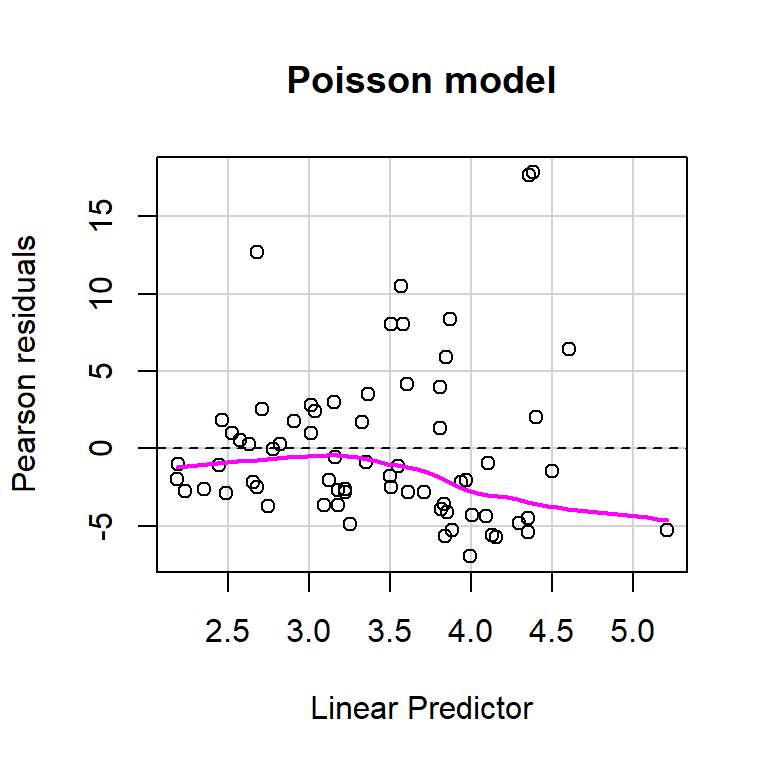

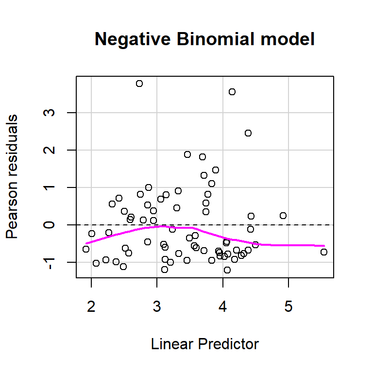
FIGURE 15.8: Plots of residuals versus each predictor and against fitted values using the residualPlots function in the car package (Fox & Weisberg, 2019).

If we also inspect the lack-of-fit tests that the residualPlots function provides, we see that they are no longer significant when using an \(\alpha = 0.05\).

residualPlots(glmNBdace, plot = FALSE)

##          Test stat Pr(>|Test stat|)  
## acreage     0.0011          0.97373  
## do2         3.5342          0.06012 .
## maxdepth    0.7947          0.37268  
## no3         0.5994          0.43882  
## so4         0.7818          0.37658  
## temp        0.4307          0.51165  
## ---
## Signif. codes:  0 '***' 0.001 '**' 0.01 '*' 0.05 '.' 0.1 ' ' 1

The residual plots created using the DHARMa package also look considerably better (Figure 15.9).

simulateResiduals(glmNBdace, plot = TRUE)

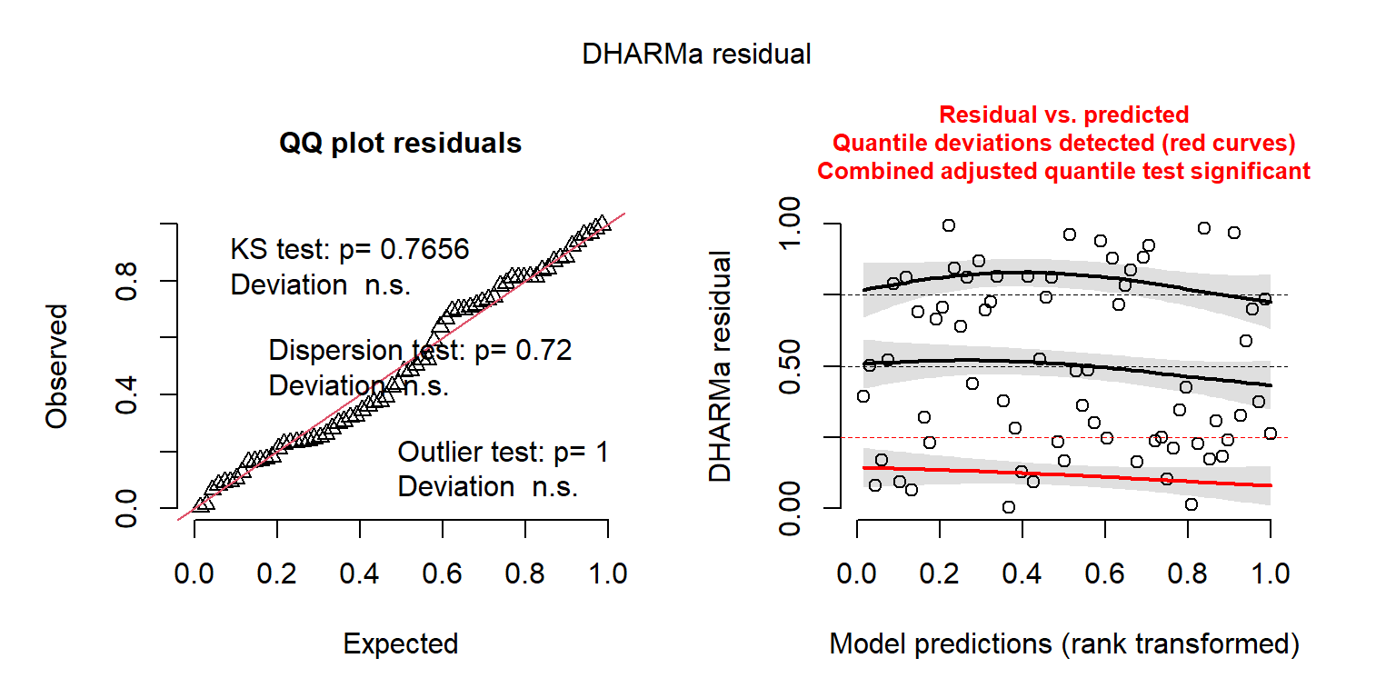
FIGURE 15.9: DHARMa residual plots for the Negative Binomial regression model fit to the longnose Dace data.

## Object of Class DHARMa with simulated residuals based on 250 simulations with refit = FALSE . See ?DHARMa::simulateResiduals for help. 
##  
## Scaled residual values: 0.3773173 0.1633754 0.7165224 0.3008422 0.7430748 0.09302904 0.8364012 0.7353561 0.1040051 0.08157994 0.3730739 0.6921645 0.3056959 0.7268539 0.2269988 0.8131921 0.2621316 0.8125872 0.2311693 0.1811807 ...

Lastly, we can adapt the goodness-of-fit test from Section 15.4.5 to the Negative Binomial model. To do so, we will assume the sampling distributions of \(\hat{\beta}\) and \(\hat{\theta}\) are independent. We can access the value of \(\hat{\theta}\) and its estimated standard error using glmNBdace$theta and glmNBdace$SE.theta, respectively. We then just need to slightly modify the calculation of the Pearson \(\chi^2\) statistic to use the correct formulas for the mean and variance.

# Number of simulations
  nsims <- 10000

# Set up matrix to hold goodness-of-fit statistics
  gfit.sim <- gfit.obs <- matrix(NA, nsims, 1)
  nobs <- nrow(longnosedace) # number of observations
  
# Extract the estimated coefficients and their asymptotic variance/covariance matrix  
# Use these values to generate nsims new betas and thetas 
  beta.hat <- MASS::mvrnorm(nsims, coef(glmNBdace), vcov(glmNBdace))
  theta.hat <- rnorm(nsims, glmNBdace$theta,  glmNBdace$SE.theta)

# Design matrix for creating new mu hats    
  xmat <- model.matrix(glmNBdace)
  for(i in 1:nsims){

    # Generate E[Y|X] and var[Y|X], mu.hat and var.hat below    
    mu.hat <- exp(xmat%*%beta.hat[i,])
    var.hat <- mu.hat + mu.hat^2/theta.hat[i]
      
    # Generate new simulated values
    new.y<-rnbinom(nobs, mu = mu.hat, size = theta.hat[i])
   
    # Calculate goodness-of-fit statistics
    gfit.sim[i,] <- sum((new.y - mu.hat)^2/(var.hat))
    gfit.obs[i, ] <- sum((longnosedace$longnosedace - mu.hat)^2/var.hat)
  }
  # Calculate and print the p-value
  (GOF.pvalue <- mean(gfit.sim > gfit.obs))

## [1] 0.2311

The p-value here is much larger, and suggests we do not have significant evidence to suggest that the Negative Binomial model is not appropriate for the data.

15.7 Model comparisons

Having settled on using a Negative Binomial model, we might now wonder if we can simplify our model at all by dropping one or more predictors. Again, my general modeling philosophy is to avoid model selection, preferring instead to report all coefficients and their standard errors in a full model (Giudice et al., 2012; Fieberg & Johnson, 2015). On the other hand, there may be reasons for performing statistical hypothesis tests, particularly with experimental data.

For large samples, difference in deviances for nested models will be distributed according to a \(\chi^2_{df}\) distribution, with df = difference in number of parameters:

\[D_2-D_1 \sim \chi^2_{p_1-p_2}\]

For quasi-Poisson models, we would need to divide the deviances by the overdispersion parameter, \(\phi\):

\[\frac{D_2-D_1}{\phi} \sim \chi^2_{p_1-p_2}\]

We can use drop1(model, test="Chi") (equivalent to a likelihood ratio test) or Anova in the car package to perform these tests. We can also use forward, backwards, stepwise selection (with the same potential issues that we discussed in Chapter 8) .

Anova(glmNBdace)

## Analysis of Deviance Table (Type II tests)
## 
## Response: longnosedace
##          LR Chisq Df Pr(>Chisq)    
## acreage   15.1095  1  0.0001015 ***
## do2        8.7214  1  0.0031449 ** 
## maxdepth   8.3963  1  0.0037598 ** 
## no3       15.5085  1  8.214e-05 ***
## so4        0.0227  1  0.8801254    
## temp       7.5073  1  0.0061448 ** 
## ---
## Signif. codes:  0 '***' 0.001 '**' 0.01 '*' 0.05 '.' 0.1 ' ' 1

The tests above are “Type II tests” of whether the coefficient with each variable is 0 in a model containing all of the other variables (Section 3.10). These tests suggest it would be reasonable to drop sO4. Alternatively, we can use AIC = -2(logL(\(\theta|y\))) + 2\(p\) for model selection with the advantage that it allows us to compare non-nested models. If we apply the stepAIC function to our Negative Binomial model, we see that it suggests dropping so4 from the model. On the other hand, it may be preferable to stick with the full model and report confidence intervals associated with all of our predictor variables (see discussion in Chapter 8).

MASS::stepAIC(glmNBdace)

## Start:  AIC=608.18
## longnosedace ~ acreage + do2 + maxdepth + no3 + so4 + temp
## 
##            Df    AIC
## - so4       1 606.20
## <none>        608.18
## - temp      1 613.35
## - maxdepth  1 614.13
## - do2       1 614.48
## - acreage   1 619.98
## - no3       1 620.32
## 
## Step:  AIC=606.2
## longnosedace ~ acreage + do2 + maxdepth + no3 + temp
## 
##            Df    AIC
## <none>        606.20
## - temp      1 611.35
## - do2       1 612.53
## - maxdepth  1 612.90
## - acreage   1 618.17
## - no3       1 618.57

## 
## Call:  MASS::glm.nb(formula = longnosedace ~ acreage + do2 + maxdepth + 
##     no3 + temp, data = longnosedace, init.theta = 1.666387265, 
##     link = log)
## 
## Coefficients:
## (Intercept)      acreage          do2     maxdepth          no3         temp  
##  -2.977e+00    4.632e-05    3.422e-01    9.660e-03    2.069e-01    9.447e-02  
## 
## Degrees of Freedom: 67 Total (i.e. Null);  62 Residual
## Null Deviance:       127.6 
## Residual Deviance: 73.65     AIC: 608.2

15.8 Bayesian implementation of count-based regression models

One of the main reasons to cover Bayesian methods is pedagogical. Fitting a model in JAGS requires that one clearly specify the model, including:

1. The likelihood, and hence the distribution of the response variable.
2. The relationship between the response and predictor variables.

In addition, as we saw in Chapter 13, it is easy to quantify uncertainty associated with average responses at a given set of predictor variables, \(E[Y_i|X_i = x_i]\), as well as uncertainty associated with new observations (i.e., confidence intervals and prediction intervals, respectively). It is equally easy to estimate uncertainty associated with functions of parameters, whereas with maximum likelihood, we had to use the delta method and rely on large sample confidence intervals (see Section 10.7).

15.8.1 Poisson regression

The code, below, can be used to implement the Poisson regression model and also conduct the goodness-of-fit test based on the Pearson \(\chi^2\) statistic. We use a shortcut to specify the linear predictor. Specifically, we pass the matrix of predictor variables and use the inprod function to multiply this matrix by a set of regression coefficients, beta. I.e., we use inprod(beta[], x[i,]) to calculate the linear predictor:

\[\log(\lambda_i) = \beta_0+\beta_1 Acreage_i+ \beta_2 DO2_i + \beta_3 maxdepth_i + \beta_4 NO3_i + \beta_5 SO4_i +\beta_6 temp_i\]

library(R2jags) 

#' Fit Poisson model using JAGS  
pois.fit<-function(){

  # Priors for regression parameters
  for(i in 1:np){
    beta[i] ~ dnorm(0,0.001)
  }  
  for(i in 1:n){
    log(lambda[i]) <- inprod(beta[], x[i,])
    longnosedace[i] ~ dpois(lambda[i])

  # Fit assessments
    Presi[i] <- (longnosedace[i] - lambda[i]) / sqrt(lambda[i]) # Pearson residuals
    dace.new[i] ~ dpois(lambda[i])    # Replicate data set
    Presi.new[i] <- (dace.new[i] - lambda[i]) / sqrt(lambda[i]) # Pearson residuals
    D[i] <- pow(Presi[i], 2)
    D.new[i] <- pow(Presi.new[i], 2)
 }

# Add up discrepancy measures
 fit <- sum(D[])
 fit.new <- sum(D.new[])
} 
  

# Bundle data
jagsdata <- list(x = xmat, np = length(coef(glmPdace)),
                 n = nrow(longnosedace), 
                 longnosedace = longnosedace$longnosedace)


# Parameters to estimate
params <- c("beta", "lambda", "Presi", "fit", "fit.new", "dace.new")


# Start Gibbs sampler
out.pois <- jags.parallel(data = jagsdata, parameters.to.save = params, 
                 model.file = pois.fit, n.thin = 2, n.chains = 3, n.burnin = 5000, 
                 n.iter = 20000)

We inspect posterior summaries for \(\beta_0\) through \(\beta_6\). This is made easier using the MCMCvis package.

library(MCMCvis)
# Look at results for the regression coefficients
MCMCsummary(out.pois, params="beta", round=3)

##           mean    sd   2.5%    50%  97.5% Rhat n.eff
## beta[1] -1.423 0.312 -2.037 -1.423 -0.822    1 14804
## beta[2]  0.000 0.000  0.000  0.000  0.000    1 18777
## beta[3]  0.188 0.024  0.140  0.188  0.236    1 15803
## beta[4]  0.015 0.001  0.013  0.015  0.016    1 16616
## beta[5]  0.191 0.011  0.170  0.191  0.214    1 17044
## beta[6] -0.004 0.004 -0.011 -0.004  0.003    1 14933
## beta[7]  0.084 0.007  0.071  0.084  0.097    1 17310

We can inspect the fit of the model by plotting posterior means of the Pearson residuals versus fitted values (Figure 15.10). We see a tendency for the Pearson residuals to increase as we move from left to right, again suggesting that we have not fully accounted for non-constant variance.

bresids <- MCMCpstr(out.pois, params = "Presi", func = mean)$Presi
bfitted <- MCMCpstr(out.pois, params = "lambda", func = mean)$lambda
jagsPfit <- data.frame(resid = bresids, fitted = bfitted)
ggplot(jagsPfit, aes(fitted, resid)) + geom_point() + 
         geom_hline(yintercept = 0) + geom_smooth() +
     xlab("Fitted value") + ylab("Pearson Residual")

## `geom_smooth()` using method = 'loess' and formula = 'y ~ x'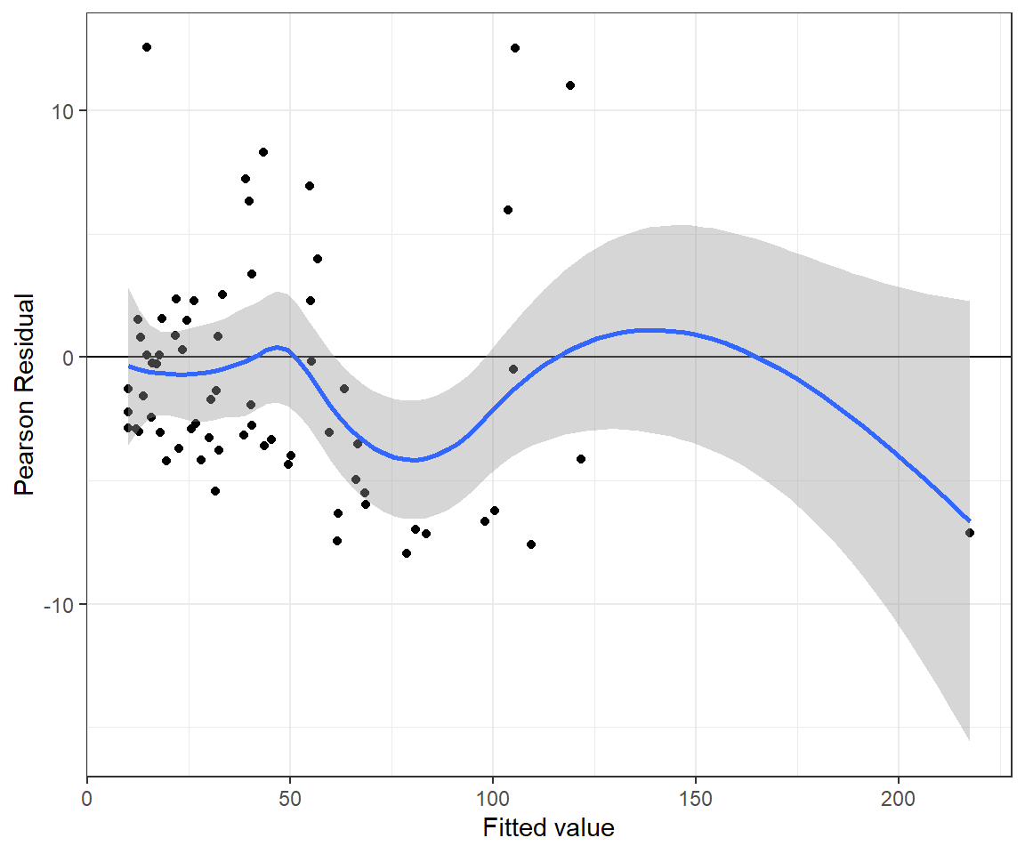

FIGURE 15.10: Pearson residuals versus fitted values for the Bayesian Poisson regression model fit to the longnose dace data.

The Bayesian p-value for the goodness-of-fit test is again \(\approx 0\). Thus, we come to the same conclusion as when fitting the model using glm; namely, the Poisson model does not fit the data very well.

fitstats <- MCMCpstr(out.pois, params = c("fit", "fit.new"), type = "chains") 
T.extreme <- fitstats$fit.new >= fitstats$fit
(p.val <- mean(T.extreme))

## [1] 0

15.8.2 Negative Binomial regression

In order to fit the Negative Binomial model in JAGS, we have to remember that the negative binomial distribution is parameterized differently in JAGS than in R. In R, we have two possible parameterizations of the Negative Binomial distribution:

• dnbinom, with parameters (prob= p, size = \(n\)) or (mu= \(\mu\), size= \(\theta\))

In JAGS, the Negative Binomial model is parameterized as:

• dnegbin with parameters (\(p\), \(\theta\))

When specifying the model in JAGS, we can write out the model in terms of \(\mu\) and \(\theta\), but then we need to solve for \(p = \frac{\theta}{\theta+\mu}\) and pass \(p\) and \(\theta\) to the dnegbin function. We also need to modify the Pearson residuals to use the variance of the Negative Binomial distribution, \(\mu+\frac{\mu^2}{\theta}\).

  #' Fit negative binomial model using JAGS  
nb.fit<-function(){

  # Priors for regression parameters
  for(i in 1:np){
    beta[i] ~ dnorm(0,0.001)
  }  
  theta~dunif(0,50)
  for(i in 1:n){
    log(mu[i]) <- inprod(beta[], x[i,])
    p[i] <- theta/(theta+mu[i])
    longnosedace[i] ~ dnegbin(p[i],theta)

  # Fit assessments
    Presi[i] <- (longnosedace[i] - mu[i]) / sqrt(mu[i]+mu[i]*mu[i]/theta) # Pearson residuals
    dace.new[i] ~ dnegbin(p[i],theta)    # Replicate data set
    Presi.new[i] <- (dace.new[i] - mu[i]) / sqrt(mu[i]+mu[i]*mu[i]/theta) # Pearson residuals
    D[i] <- pow(Presi[i], 2)
    D.new[i] <- pow(Presi.new[i], 2)
 }

# Add up discrepancy measures
 fit <- sum(D[])
 fit.new <- sum(D.new[])
} 
  

# Parameters to estimate
params <- c("mu", "beta", "theta","Presi", "fit", "fit.new", "dace.new")


# Start Gibbs sampler
out.nb <- jags.parallel(data = jagsdata, parameters.to.save = params, 
               model.file = nb.fit, n.thin = 2, n.chains = 3, n.burnin = 5000, 
                 n.iter = 20000)

The residual plot looks a little bit better for the Negative Binomial model (Figure 15.11) and the p-value for the goodness-of-fit test is now much larger than 0.05.

nbresids <- MCMCpstr(out.nb, params = "Presi", func = mean)$Presi
nbfitted <- MCMCpstr(out.nb, params = "mu", func = mean)$mu
jagsnbfit <- data.frame(resid = nbresids, fitted = nbfitted)
ggplot(jagsnbfit, aes(fitted, resid)) + geom_point() + 
         geom_hline(yintercept = 0) + geom_smooth() +
     xlab("Fitted value") + ylab("Pearson Residual")

## `geom_smooth()` using method = 'loess' and formula = 'y ~ x'

FIGURE 15.11: Pearson residuals versus fitted values for the Negative Binomial regression model fit to the longnose dace data.

fitstats <- MCMCpstr(out.nb, params = c("fit", "fit.new"), type = "chains") 
T.extreme <- fitstats$fit.new >= fitstats$fit
(p.val <- mean(T.extreme))

## [1] 0.3171111

Lastly, for fun, we compare the frequentist and Bayesian 95% confidence/credible intervals for the Negative Binomial Model (Figure 15.12).

# Summary of the Bayesian model
Nbsum<-MCMCsummary(out.nb, params=c("beta","theta"), round=3)

# Confidence intervals Frequentist model
ci.nb<-confint(glmNBdace)

# Create data frame with results
est.dat<-data.frame(
  bhat = c(Nbsum[, 1], coef(glmNBdace), glmNBdace$theta),
  lowci = c(Nbsum[, 3], ci.nb[, 1], glmNBdace$theta - 1.96 * glmNBdace$SE.theta),
  upci = c(Nbsum[, 5], ci.nb[, 2], glmNBdace$theta + 1.96 * glmNBdace$SE.theta),
  Method = c(rep("Freq", 8), rep("Bayes", 8)),
  coefname = rep(c(names(coef(glmNBdace)), "theta"), 2))

ggplot(est.dat, aes(coefname, bhat, colour = Method)) + 
  geom_point(size = 5, shape = 18, position = position_dodge(width = 0.5)) +
  geom_errorbar(aes(ymax = upci, ymin = lowci, colour = Method),
      position = position_dodge(width = 0.5)) + ylab("Point Estimate") +
  xlab("Coefficient") +  scale_colour_colorblind()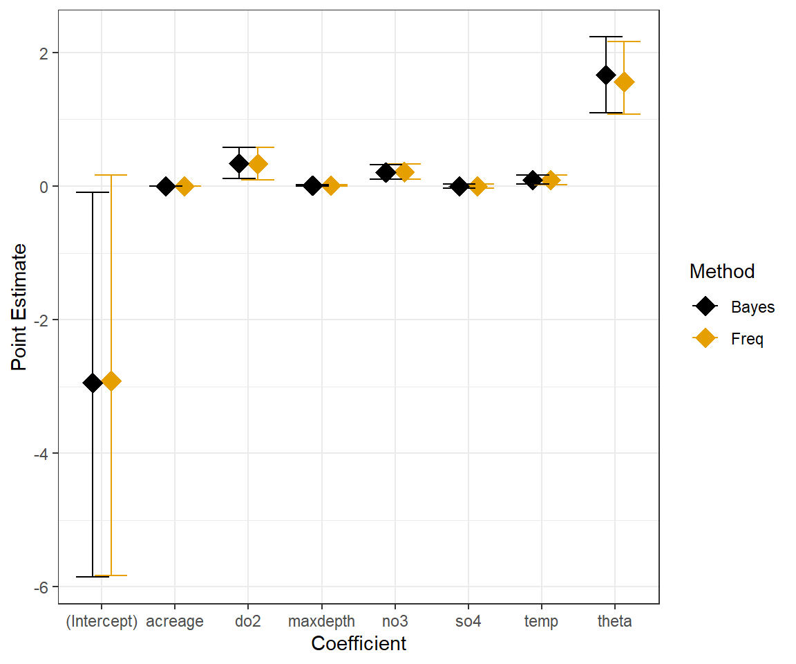

FIGURE 15.12: Comparison of frequentist and Bayesian Negative Binomial Models fit to longnose dace data.

15.8.3 Poisson-Normal model

Another alternative model that is sometimes considered for overdispersed data is a Poisson-Normal model (Harrison, 2014):

\[Y_i | X_i, \epsilon_i \sim Poisson(\lambda_i)\]

\[log(\lambda_i) = \log(\mu_i) = \beta_0 + \beta_1x_1 + \ldots \beta_px_p + \epsilon_i\]

\[\epsilon_i \sim N(0, \sigma^2)\]

In order to calculate the mean and variance of \(Y_i|X_i\), we have to integrate over the distribution of \(\epsilon_i\), which leads us to the following expressions:

• \(E[Y_i|X_i] = e^{\beta_0 + \beta_1X_{1,i} + \ldots \beta_pX_{p,i} + \frac{1}{2}\sigma^2}\)
  
• \(Var[Y_i|X_i] = \mu_i + (e^{\sigma^2}-1)\mu_i^2\)

Note, that the expression for the mean is not the same as \(E[Y|X, \epsilon = 0] = \exp^{\beta_0 + \beta_1X_1 + \ldots \beta_pX_p}\). We will encounter similar complexities when we include random effects on the link scale to model correlation among repeated measures on the same sample units (Chapter 19).

Below, I fit this model to the dace data:

#' Fit Poisson model using JAGS  
poisnorm.fit<-function(){

  # Priors for regression parameters
  for(i in 1:np){
    beta[i] ~ dnorm(0,0.001)
  }  
  
  # Prior for sigma and tau
  sig ~ dunif(0, 3) 
  tau <- 1/(sig*sig)
  
  
  for(i in 1:n){
  # Likelihood
    log(lambda[i]) <- inprod(beta[], x[i,]) + eps[i]
    longnosedace[i] ~ dpois(lambda[i])
    eps[i] ~ dnorm(0, tau)
    
  # Calculate mean and variance
    mu[i] <-  exp(inprod(beta[], x[i,]) + sig^2/2)
    vary[i] <- mu[i] + (exp(sig^2)-1)*mu[i]^2
     
  # Fit assessments
    Presi[i] <- (longnosedace[i] - mu[i]) / sqrt(vary[i]) # Pearson residuals
    dace.new[i] ~ dpois(lambda[i])    # Replicate data set
    Presi.new[i] <- (dace.new[i] - mu[i]) / sqrt(vary[i]) # Pearson residuals
    D[i] <- pow(Presi[i], 2)
    D.new[i] <- pow(Presi.new[i], 2)
 }

# Add up discrepancy measures
 fit <- sum(D[])
 fit.new <- sum(D.new[])
} 
  
# Parameters to estimate
params <- c("beta", "mu", "Presi", "fit", "fit.new")


# Start Gibbs sampler
out.poisnorm <- jags.parallel(data = jagsdata, parameters.to.save = params, 
                 model.file = poisnorm.fit, n.thin = 2, n.chains = 3, n.burnin = 5000, 
                 n.iter = 20000)

The residual versus fitted value plot for the Poisson-Normal model looks reasonable (Figure 15.13).

pnresids <- MCMCpstr(out.poisnorm, params = "Presi", func = mean)$Presi
pnfitted <- MCMCpstr(out.poisnorm, params = "mu", func = mean)$mu
jagspnfit <- data.frame(resid = pnresids, fitted = pnfitted)
ggplot(jagspnfit, aes(fitted, resid)) + geom_point() + 
         geom_hline(yintercept = 0) + geom_smooth() +
     xlab("Fitted value") + ylab("Pearson Residual")

## `geom_smooth()` using method = 'loess' and formula = 'y ~ x'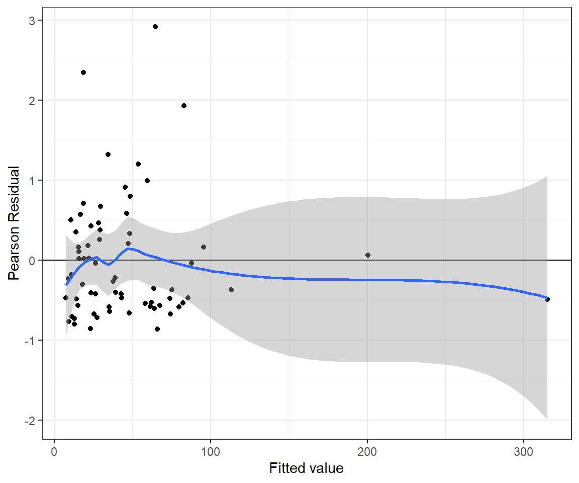

FIGURE 15.13: Pearson residuals versus fitted values for the Poisson-Normal regression model fit to the longnose dace data.

In addition, the Bayesian p-value is close to 0.5, suggesting the Poisson-Normal model is a reasonable data generating model for these data.

fitstats <- MCMCpstr(out.poisnorm, params = c("fit", "fit.new"), type = "chains") 
T.extreme <- fitstats$fit.new >= fitstats$fit
(p.val <- mean(T.extreme))

## [1] 0.5211556

15.8.4 Aside: Bayesian model selection

There are several information criterion available for comparing models fit using Bayesian methods (see e.g., Hooten & Hobbs, 2015 for a review). One of the most popular, though perhaps not the most appropriate, is DIC = Deviance Information Criterion.

Recall, the deviance, D = -2\(logL(\theta | y)\). In Bayesian implementations, the fact that we have a posterior distribution for our parameters, \(\theta\), means that we also have a posterior distribution of the deviance. DIC is calculated from:

• \(\overline{D}\) = the mean of the posterior deviance
• \(\hat{D}\) = the deviance calculated using the posterior means of the different model parameters

DIC uses the difference between these two quantities to estimate the effective number of parameters in a model, \(p_D=\overline{D}-\hat{D}\). DIC is then estimated using:

DIC = \(\hat{D} + 2p_D = (\overline{D}-p_D)+2p_D = \overline{D}+p_D\)

JAGS reports DIC in its summary, which can also be accessed as follows:

out.pois$BUGSoutput$DIC

## [1] 2474.525

out.nb$BUGSoutput$DIC

## [1] 610.9902

out.poisnorm$BUGSoutput$DIC

## [1] 473.6137

These results mirror the AIC comparison between the Poisson and Negative Binomial model but also suggest that the Poisson-Normal model may offer the best fit to the data.

15.8.5 Cautionary statements regarding DIC

DIC is not without problems. Here is what Martyn Plummer, the creator of JAGS has to say:

The deviance information criterion (DIC) is widely used for Bayesian model comparison, despite the lack of a clear theoretical foundation….valid only when the effective number of parameters in the model is much smaller than the number of independent observations. In disease mapping, a typical application of DIC, this assumption does not hold and DIC under-penalizes more complex models. Another deviance-based loss function, derived from the same decision-theoretic framework, is applied to mixture models, which have previously been considered an unsuitable application for DIC.

And, Andrew Gelman had this to say:

I don’t really ever know what to make of DIC. On one hand, it seems sensible…On the other hand, I don’t really have any idea what I would do with DIC in any real example. In our book we included an example of DIC–people use it and we don’t have any great alternatives–but I had to be pretty careful that the example made sense. Unlike the usual setting where we use a method and that gives us insight into a problem, here we used our insight into the problem to make sure that in this particular case the method gave a reasonable answer.

There are other options for comparing models fit in a Bayesian framework. Two popular options are LOO (Vehtari & Lampinen, 2002) and WAIC (Watanabe & Opper, 2010), which are available in the loo package (Vehtari et al., 2020). Again, I recommend reading Hooten & Hobbs (2015) to learn more about these metrics; see also Vehtari, Gelman, & Gabry (2017).

15.9 Modeling rates and densities using an offset

Count data are often collected over varying lengths of time or in sample units that have different areas. We can account for variable survey effort by modeling rates (counts per unit time) or densities (counts per unit area) using Poisson or Negative Binomial regression with an offset. Example applications include models of catch per unit effort (CPUE) in fisheries applications (e.g., Z. Su & He, 2013), encounter rates in camera-trap studies (e.g., Scotson, Fredriksson, Ngoprasert, Wong, & Fieberg, 2017), and visitation rates in pollinator studies (Reitan & Nielsen, 2016).

An offset is like a special predictor variable where we set its regression coefficient to 1. To see how this works, consider a model for the log(rate) as a linear function of predictors:

\(\log(E[Y_i|X_i]/\mbox{Time}) = \beta_0 + \beta_1X_{1,i} + \ldots+ \beta_pX_{p,i}\)

\(\Rightarrow \log(E[Y_i|X_i]) - \log(\mbox{Time}) = \beta_0 + \beta_1X_{1,i} + \ldots+ \beta_pX_{p,i}\)

\(\Rightarrow \log(E[Y|X]) = \log(\mbox{Time}) + \beta_0 + \beta_1X_{1,i} + \ldots+ \beta_pX_{p,i}\)

We can include \(\log(\mbox{Time})\) as an offset, e.g., using R:

glm(y~x + offset(log(time)), data= , family = poisson())

This ensures that \(\log(\mbox{Time})\) is taken into account when estimating the other regression coefficients, but we do not estimate a coefficient for \(\log(\mbox{Time})\). We can think of this model as one for the rate, or alternatively, a model for the count where the mean count is determined by a rate parameter, \(\lambda_i\), multiplied by the total effort, \(E_i\), such that \(E[Y_i|X_i] =\lambda_iE_i\).

What are the advantages to modelling a rate using a count distribution (Poisson or negative binomial) with an offset rather than modeling the rate directly using a continuous statistical distribution (e.g., log-normal)? First, the log-normal distribution cannot handle 0’s, so many users will add a small constant, \(c\), and model \(\log(Y + c)\) (O’Hara & Kotze, 2010), but results may be sensitive to the size of this constant. Furthermore, we lose some information by modeling the rates directly. Consider two observations that have a 0 count, but one observation has twice the effort of the other observation. If we model the count divided by effort, both observations are treated identically (since in both cases \(y_i\) = 0). The rate model, by contrast, will naturally account for the differing levels of effort.

Although modeling rates and densities is often appealing, it may be useful to consider including a measure of log(effort) as a covariate first. When the regression coefficient for log(effort) is close to 1, then it can safely be replaced with an offset. If the coefficient is far from 1, however, it may be preferable to retain the covariate.

To demonstrate this approach, we consider catch and effort data of black sea bass (Centropristis striata) from the Southeast Reef Fish Survey. The data are contained in reeffish within the Data4Ecologists package.

data(reeffish)
head(reeffish)

##   Year      Date  Time Doy Hour Duration Temperature Depth Seabass
## 1 1998 7/23/1998 11:50 204   12       97    9.495300    53       0
## 2 1998 7/23/1998 11:53 204   12      101    9.495300    52       0
## 3 1998 7/23/1998 13:56 204   14       96    9.548500    52       0
## 4 1998 7/23/1998 18:11 204   18       89    9.750867    52       0
## 5 1998 7/23/1998 18:18 204   18       91    9.750867    47       0
## 6 1998 7/23/1998 18:34 204   19       91    9.750867    52       0

The data set contains a count of sea bass (Seabass) captured in Chevron traps, along with the sampling duration (in minutes) associated with each observation (Duration) for surveys conducted between 1990 and 2021. Potential predictor variables include Julian date (Doy), hour of the day (Hour), temperature (Temperature), and water depth (Depth). We might also expect catch-per-unit effort to vary annually, and thus, we will include Year as a categorical variable⁶⁴. We will consider a quadratic function to model a non-linear effect of Temperature on the log scale.

The data from the survey are highly variable, with many observations of 0 sea bass in the trap⁶⁵. A Poisson model fit to the data will fail to pass standard goodness-of-fit tests, so we will go directly to fitting the following Negative Binomial model using glm.nb in the MASS package (Venables & Ripley, 2002):

\[\begin{gather} C_{i,t} \sim \text{Negative Binomial}(\lambda_{i,t}E_{i,t}, \theta) \nonumber \\ \log(\lambda_i E_{i,t}) = \beta_{0,t} + \beta_1 Temperature_{i,t} + \beta_2 Temperature^2_{i,t} + \nonumber \\ \beta_3Depth_{i,t} + \beta_4Doy_{i,t} + \beta_5Hour_{i,t} \nonumber \end{gather}\]

Here, \(C_{i,t}\) and \(E_{i,t}\) are the catch and effort (sampling duration) associated with the \(i^{th}\) observation in year \(t\), \(\lambda_{i,t}\) is the expected catch per unit effort in the survey, and \(\theta\) is an overdispersion parameter of the Negative Binomial distribution. Note, we have written the model as though fit using a means parameterization for Year so that we can simply capture the different intercepts in each year with the term \(\beta_{0,t}\). We can fit the model using:

reeffish <- reeffish %>% mutate(logduration = log(Duration))
fitoffset <- glm.nb(Seabass ~ as.factor(Year) + poly(Temperature,2) + 
                      Depth + Doy + Hour + offset(logduration) -1, data = reeffish)
summary(fitoffset)

## 
## Call:
## glm.nb(formula = Seabass ~ as.factor(Year) + poly(Temperature, 
##     2) + Depth + Doy + Hour + offset(logduration) - 1, data = reeffish, 
##     init.theta = 0.2529787278, link = log)
## 
## Coefficients:
##                         Estimate Std. Error z value Pr(>|z|)    
## as.factor(Year)1990    2.259e+00  1.594e-01  14.174  < 2e-16 ***
## as.factor(Year)1991    1.949e+00  1.778e-01  10.960  < 2e-16 ***
## as.factor(Year)1992    2.010e+00  1.637e-01  12.280  < 2e-16 ***
## as.factor(Year)1993    1.723e+00  1.613e-01  10.687  < 2e-16 ***
## as.factor(Year)1994    1.614e+00  1.657e-01   9.740  < 2e-16 ***
## as.factor(Year)1995    1.426e+00  1.693e-01   8.426  < 2e-16 ***
## as.factor(Year)1996    1.686e+00  1.680e-01  10.038  < 2e-16 ***
## as.factor(Year)1997    1.700e+00  1.685e-01  10.087  < 2e-16 ***
## as.factor(Year)1998    1.728e+00  1.615e-01  10.698  < 2e-16 ***
## as.factor(Year)1999    2.201e+00  1.882e-01  11.701  < 2e-16 ***
## as.factor(Year)2000    2.015e+00  1.783e-01  11.301  < 2e-16 ***
## as.factor(Year)2001    2.433e+00  1.847e-01  13.174  < 2e-16 ***
## as.factor(Year)2002    1.229e+00  1.943e-01   6.326 2.51e-10 ***
## as.factor(Year)2003    6.698e-01  2.054e-01   3.261  0.00111 ** 
## as.factor(Year)2004    2.339e+00  1.795e-01  13.031  < 2e-16 ***
## as.factor(Year)2005    1.777e+00  1.745e-01  10.184  < 2e-16 ***
## as.factor(Year)2006    1.967e+00  1.772e-01  11.098  < 2e-16 ***
## as.factor(Year)2007    1.446e+00  1.739e-01   8.318  < 2e-16 ***
## as.factor(Year)2008    1.563e+00  1.789e-01   8.740  < 2e-16 ***
## as.factor(Year)2009    1.258e+00  1.622e-01   7.757 8.71e-15 ***
## as.factor(Year)2010    2.530e+00  1.462e-01  17.302  < 2e-16 ***
## as.factor(Year)2011    2.700e+00  1.446e-01  18.678  < 2e-16 ***
## as.factor(Year)2012    2.666e+00  1.331e-01  20.026  < 2e-16 ***
## as.factor(Year)2013    2.376e+00  1.303e-01  18.234  < 2e-16 ***
## as.factor(Year)2014    2.091e+00  1.276e-01  16.390  < 2e-16 ***
## as.factor(Year)2015    1.754e+00  1.288e-01  13.620  < 2e-16 ***
## as.factor(Year)2016    1.492e+00  1.355e-01  11.014  < 2e-16 ***
## as.factor(Year)2017    1.287e+00  1.280e-01  10.049  < 2e-16 ***
## as.factor(Year)2018    1.110e+00  1.245e-01   8.913  < 2e-16 ***
## as.factor(Year)2019    6.354e-01  1.276e-01   4.981 6.32e-07 ***
## as.factor(Year)2021   -1.408e-01  1.245e-01  -1.131  0.25811    
## poly(Temperature, 2)1 -3.263e+01  2.959e+00 -11.028  < 2e-16 ***
## poly(Temperature, 2)2  1.818e+01  2.343e+00   7.760 8.48e-15 ***
## Depth                 -1.388e-01  1.535e-03 -90.451  < 2e-16 ***
## Doy                    5.426e-04  4.359e-04   1.245  0.21317    
## Hour                   8.856e-03  4.679e-03   1.893  0.05839 .  
## ---
## Signif. codes:  0 '***' 0.001 '**' 0.01 '*' 0.05 '.' 0.1 ' ' 1
## 
## (Dispersion parameter for Negative Binomial(0.253) family taken to be 1)
## 
##     Null deviance: 43485  on 21039  degrees of freedom
## Residual deviance: 16826  on 21003  degrees of freedom
## AIC: 89995
## 
## Number of Fisher Scoring iterations: 1
## 
## 
##               Theta:  0.25298 
##           Std. Err.:  0.00361 
## 
##  2 x log-likelihood:  -89921.25400

If we look at the coefficients in the summary of the model, we see that we do not estimate a coefficient for log(Duration). Yet, this information is accounted for in the model by including the offset(log(Duration)) term, which allows us to model the catch rate rather than the count of sea bass observed.

We could also fit a model that includes log(Duration) as a predictor. We can examine the coefficient for log(Duration) and also compare the two models using AIC to determine if the latter model does a better job of fitting the data than the catch-rate model.

fitpredictor <- glm.nb(Seabass ~ as.factor(Year) + poly(Temperature,2) + 
                      Depth + Doy + Hour + logduration -1, data = reeffish)
AIC(fitoffset, fitpredictor)

##              df      AIC
## fitoffset    37 89995.25
## fitpredictor 38 89996.88

# Profile-likelihood confidence interval
round(confint(fitpredictor, parm = "logduration"), 2)

## Waiting for profiling to be done...

##  2.5 % 97.5 % 
##   0.65   1.19

In this case, we see that AIC slightly prefers the model with the offset. Further, the confidence interval for the coefficient associated with log(Duration) includes 1. Thus, we have support for using the simpler model, which also has the advantage of interpretation – i.e., we can simply state that we are modeling the catch per unit effort. We end by using effect plots, constructed using the ggpredict package, to visualize the importance of the predictors (Figure 15.14). These plots depict estimates of adjusted means formed varying a focal predictor (shown on the x-axis) while holding all other predictor variables at their sample means (Section 3.14.3). We see that the effects of depth and temperature far outweigh those of the other variables.

sjPlot::plot_grid(plot(ggpredict(fitoffset),  one_plot = FALSE))

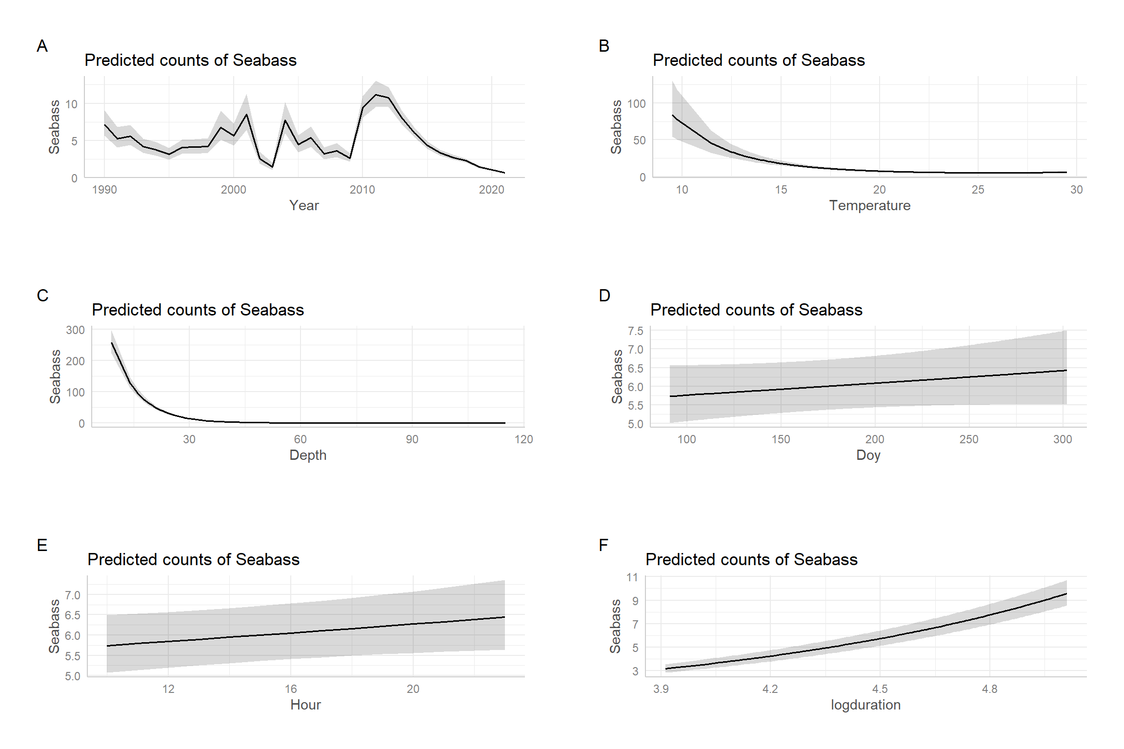
FIGURE 15.14: Effect plots depicting estimates of marginal means for the Negative Binomial regression model fit to the black sea bass data.

References

Arel-Bundock, V. (2022). modelsummary: Data and model summaries in R. Journal of Statistical Software, 103(1), 1–23. doi:10.18637/jss.v103.i01

Faraway, J. J. (2016). Extending the linear model with r: Generalized linear, mixed effects and nonparametric regression models. CRC press.

Fieberg, J., & Johnson, D. H. (2015). MMI: Multimodel inference or models with management implications? The Journal of Wildlife Management, 79(5), 708–718.

Fox, J., & Weisberg, S. (2019). An R companion to applied regression (Third). Thousand Oaks CA: Sage. Retrieved from https://socialsciences.mcmaster.ca/jfox/Books/Companion/

Giudice, J. H., Fieberg, J., & Lenarz, M. S. (2012). Spending degrees of freedom in a poor economy: A case study of building a sightability model for moose in northeastern minnesota. The Journal of Wildlife Management, 76(1), 75–87.

Harrison, X. A. (2014). Using observation-level random effects to model overdispersion in count data in ecology and evolution. PeerJ, 2, e616.

Hartig, F. (2021). DHARMa: Residual diagnostics for hierarchical (multi-level / mixed) regression models. Retrieved from https://CRAN.R-project.org/package=DHARMa

Hooten, M. B., & Hobbs, N. T. (2015). A guide to bayesian model selection for ecologists. Ecological Monographs, 85(1), 3–28.

Kéry, M. (2010). Introduction to WinBUGS for ecologists: Bayesian approach to regression, ANOVA, mixed models and related analyses. Academic Press.

Lüdecke, D., Ben-Shachar, M. S., Patil, I., Waggoner, P., & Makowski, D. (2021). performance: An R package for assessment, comparison and testing of statistical models. Journal of Open Source Software, 6(60), 3139. doi:10.21105/joss.03139

McCullagh, P., & Nelder, J. A. (1989). Generalized linear models, second edition. Chapman & Hall. Retrieved from http://books.google.com/books?id=h9kFH2\_FfBkC

McFadden, D. (1977). Quantitative methods for analyzing travel behavior of individuals: Some recent 857 developments: Institute of transportation studies. University of California, 858.

Nakagawa, S., & Schielzeth, H. (2013). A general and simple method for obtaining R2 from generalized linear mixed-effects models. Methods in Ecology and Evolution, 4(2), 133–142.

O’Hara, R., & Kotze, J. (2010). Do not log-transform count data. Nature Precedings, 1–1.

Reitan, T., & Nielsen, A. (2016). Do not divide count data with count data; a story from pollination ecology with implications beyond. PloS One, 11(2).

Scotson, L., Fredriksson, G., Ngoprasert, D., Wong, W.-M., & Fieberg, J. (2017). Projecting range-wide sun bear population trends using tree cover and camera-trap bycatch data. PloS One, 12(9).

Su, Y.-S., & Masanao Yajima. (2021). R2jags: Using r to run ’JAGS’. Retrieved from https://CRAN.R-project.org/package=R2jags

Su, Z., & He, J. X. (2013). Analysis of lake huron recreational fisheries data using models dealing with excessive zeros. Fisheries Research, 148, 81–89.

Vehtari, A., Gabry, J., Magnusson, M., Yao, Y., Bürkner, P.-C., Paananen, T., & Gelman, A. (2020). Loo: Efficient leave-one-out cross-validation and WAIC for bayesian models. Retrieved from https://mc-stan.org/loo/

Vehtari, A., Gelman, A., & Gabry, J. (2017). Practical bayesian model evaluation using leave-one-out cross-validation and WAIC. Statistics and Computing, 27, 1413–1432. doi:10.1007/s11222-016-9696-4

Vehtari, A., & Lampinen, J. (2002). Bayesian model assessment and comparison using cross-validation predictive densities. Neural Computation, 14(10), 2439–2468.

Venables, W. N., & Ripley, B. D. (2002). Modern applied statistics with s (Fourth). New York: Springer. Retrieved from https://www.stats.ox.ac.uk/pub/MASS4/

Warton, D. I., Lyons, M., Stoklosa, J., & Ives, A. R. (2016). Three points to consider when choosing a LM or GLM test for count data. Methods in Ecology and Evolution, 7(8), 882–890.

Watanabe, S., & Opper, M. (2010). Asymptotic equivalence of bayes cross validation and widely applicable information criterion in singular learning theory. Journal of Machine Learning Research, 11(12).

Youngflesh, C. (2018). MCMCvis: Tools to visualize, manipulate, and summarize MCMC output. Journal of Open Source Software, 3(24), 640. doi:10.21105/joss.00640

Zuur, A., Ieno, E. N., Walker, N., Saveliev, A. A., & Smith, G. M. (2009). Mixed effects models and extensions in ecology with r. Springer Science & Business Media.

---

60. Note that I have chosen to simplify the equation for the model slightly by writing \(Y_i \sim Poisson(\lambda_i)\) rather than \(Y_i |X_i \sim Poisson(\lambda_i)\). I like the former notation because it makes it clear that the distribution of the response variable depends on the predictor variables included in the model. With so many predictors, however, the equation would get a bit unwieldy if we listed them all. Also, note that we are assuming that the predictor variables are known quantities, so it is less important that we write down an equation for the distribution of \(Y_i\) as being conditional on \(X_i\). When consider models that include latent variables (Chapter 17) or random effects (Chapter 18), it will be important to explicitly acknowledge when our distribution of \(Y_i\) is conditional on specific values of these random quantities. I.e., we need to be careful to indicate if the distribution for \(Y_i\) is a conditional distribution or marginal distribution. The latter will require averaging over other random variables (i.e., the latent variables or random effects).↩︎

61. There are several R packages that can be used to create tables summarizing regression output. The tab_mod function in the sjPlots library will, by default, report rate ratios for Poisson regression models. Further, the modelsummary function in the modelsummary package (Arel-Bundock, 2022) has an argument, exponentiate = TRUE for calculating rate ratios and their confidence intervals and was used to create Table 15.2.↩︎

62. This approach is also similar to the Generalized Estimating Equation approach that we will see in Chapter 20.↩︎

63. Alternatively, one might try various transformations, including a \(\log(y +1)\) transformation and then use a linear model. For a comparison of these approaches, see Warton, Lyons, Stoklosa, & Ives (2016).↩︎

64. Alternatively, we could explore temporal trends in catch rates by modeling Year as a continuous variable. Further, we might consider modeling annual variation using random effects (see Chapters 18, 19).↩︎

65. Zero-inflation models considered in Chapter 17 would offer another alternative.↩︎