Chapter 19 Generalized linear mixed effects models (GLMMs)
Learning objectives
Learn how to implement mixed models in R for count and binary data using generalized linear mixed effect models (GLMMs)
Gain an appreciation for why generalized linear mixed effects can be difficult to fit
Understand why parameters in mixed-effects models may have a different interpretation when modeling using a non-linear link function
Learn how to estimate population-level response patterns for count and binary data using GLMMs by integrating over the distribution of the random effects
Be able to describe models and their assumptions using equations and text and match parameters in these equations to estimates in computer output.
We will begin by briefly reviewing modeling approaches that are appropriate for repeated measures data where the response variable, \(Y\), conditional on predictor variables, \(X\) is Normally distributed. These methods include linear mixed-effects models (Chapter 18) and generalized least squares (Section 18.14). We will then consider modeling approaches for repeated measures in cases where \(Y | X\) has a distribution other than a Normal distribution, including generalized linear mixed effect models (GLMMs) in this Section, and Generalized Estimating Equations (GEE) in Chapter 20. Throughout, we will draw heavily upon the material in Fieberg et al. (2009), which explores data from a study of mallard nesting structures, including the clutch size data from Chapter 4.
19.1 R packages
We begin by loading a few packages upfront:
library(tidyverse) # for data wrangling
library(gridExtra) # for multi-panel plots
library(lme4)  # for fitting random-effects models
library(nlme) # for fitting random-effect and gls models
library(glmmTMB) # for fitting random-effects models
library(modelsummary) # for creating output tables
library(kableExtra) # for tables
options(kableExtra.html.bsTable = T)
library(ggplot2)# for plotting
library(performance) # for model diagnostics
library(ggeffects) # for effect plots
In addition, we will use data and functions from the following packages:
Data4Ecologistsfor theclutchdata setGLMMadaptivefor fitting generalized linear mixed effect models and estimating marginal response patterns from themcarfor multiple degree-of-freedom hypothesis tests using theAnovafunction
19.2 Case study: A comparison of single and double-cylinder nest structures
In the late 90’s, the Minnesota Department of Natural Resources (MN DNR) conducted a study to compare the cost-effectiveness of single- and double-cylinder mallard nesting structures and to identify the best places to locate them in the landscape (Zicus et al., 2003; Zicus, Rave, Das, Riggs, & Buitenwerf, 2006; Zicus, Rave, & Fieberg, 2006). A drawing of a single cylinder structure by a former MN DNR employee, Ross Hier, who happens to be a fantastic artist is depicted below (Figure 19.1); a double-cylinder structure would have two cylinders associated with a single pole. To accomplish the project objectives, 110 nest structures (53 single-cylinder and 57 double-cylinder) were placed in 104 wetlands (the largest eight wetlands included two structures each). The structure type (single or double) was randomly chosen for each location. The nest structures were inspected \(\ge 4\) times annually from 1997-1999 to determine whether or not each nest cylinder was occupied. In addition, clutch sizes were recorded for 139 nests during the course of the study. Thus, we have multiple observations for each nest structure, and we might expect our response variables (structure occupancy or clutch size) from the same structure to be more similar than observations from different structures even after accounting for known covariates.
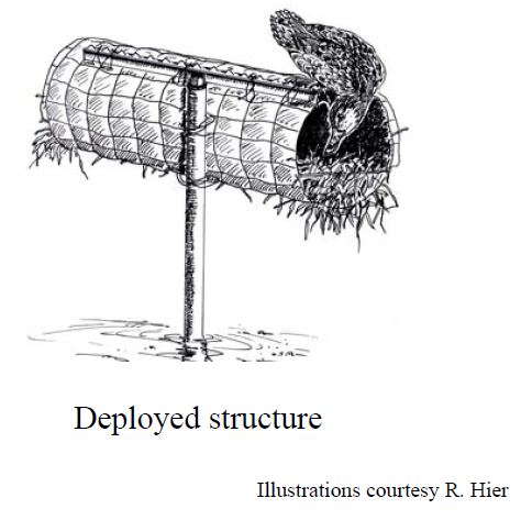
FIGURE 19.1: Single-cylinder mallard nesting structure.
19.3 Review of approaches for modeling correlated data for Normally distributed response variables.
Let’s start by considering the clutch size data. Because clutch sizes (number of eggs in the nest) are count data, it is natural to consider a Poisson or Negative Binomial regression model. Nonetheless, the counts are fairly large, and for large counts, a Normal approximation may be reasonable. Note, at the time this study was conducted, software for fitting linear mixed effects models was becoming widely available, but software for fitting generalized linear mixed effects models was not yet well developed. Thus, the analyses in Zicus et al. (2003) were conducted using linear mixed-effects models. To avoid having to model the non-linear relationship between clutch size and nest initiation date (Figure 4.1), we will drop outliers associated with nests initiated late in the season. We will also exclude observations with more than 12 eggs as these are likely associated with nests that have been parasitized.
library(Data4Ecologists) # data package
data(clutch)

# Get rid of observations with nest initiation dates > 30 May
# and a few outliers representing nests that were likely parasitized
clutch <- clutch %>% filter(CLUTCH < 13 & date < 149) %>%
  mutate(year = as.factor(year)) %>%
  mutate(Ideply = ifelse(DEPLY==2, TRUE, FALSE))
ggplot(clutch, aes(date, CLUTCH, col=Ideply))+
  geom_point() +
  geom_smooth(method= lm, formula = y ~ x) +
  facet_wrap(~year)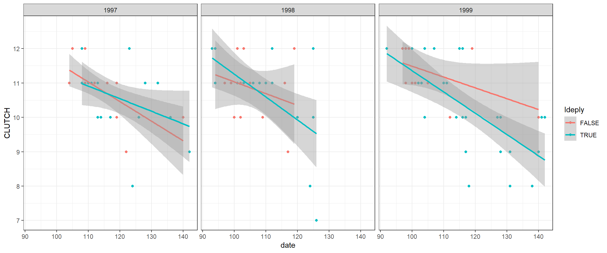
FIGURE 19.2: Clutch sizes in mallard nest boxes in Minneosta versus nest initiation date for 3 separate years and different deployment (single versus double-cylinder) types.
In this data set, we have 2 potential grouping variables, year and strtno, the latter is a unique identifier for each structure.
Think-Pair-Share: is it better to model the effect of these grouping variables (and any interactions with them) as fixed or random effects? What is the difference?
We only have data from 3 years, so it is best to model variability among years using a set of fixed effects. It would be difficult to estimate a variance parameter for year or to generalize to a larger population of years with so little data. On the other hand, we have data from 110 nest structures. It makes more sense to model variability among structures using random effects, which will also allow us to generalize our results to a larger population (of locations where we could place nest structures). Let’s consider the following model for the clutch sizes:
\[\begin{gather} Y_{ij} | b_{0i} \sim N(\mu_i, \sigma^2_{\epsilon}) \nonumber \\ \mu_i = (\beta_0 + b_{0i}) + \beta_1 Init.Date_{ij} + \beta_2I(deply=2)_i \tag{19.1} \\ b_{0i} \sim N(0, \sigma_{b0}^2), \nonumber \end{gather}\]
where \(Y_{ij}\) is the clutch size for the \(i^{th}\) structure during year \(j\), \(Init.Date_{ij}\) = the nest initiation date (Julian day) for the \(i^{th}\) structure during year \(j\), and \(I(deply=2)_{i}\) = 0 if \(i^{th}\) structure is a single cylinder, and 1 if double cylinder.
How does this model differ from a fixed effects model that might also include strtno? A fixed-effects model would use a series of dummy variables to model differences between the nest structures, allowing each structure to have its own intercept. The random effects model is similar, except that we:
- Assume the intercepts for each structure come from a common Normal distribution.
- We estimate the variance of the structure-specific intercepts, \(\sigma_{b0}^2\), rather than separate parameters for each structure (we can, however, predict structure-specific intercepts once we have estimates of the other parameters).
## Linear mixed model fit by REML ['lmerMod']
## Formula: CLUTCH ~ date + Ideply + (1 | strtno)
##    Data: clutch
##
## REML criterion at convergence: 283.2
##
## Scaled residuals:
##      Min       1Q   Median       3Q      Max
## -2.81168 -0.44368 -0.03218  0.55879  2.14321
##
## Random effects:
##  Groups   Name        Variance Std.Dev.
##  strtno   (Intercept) 0.2532   0.5032
##  Residual             0.5755   0.7586
## Number of obs: 106, groups:  strtno, 52
##
## Fixed effects:
##              Estimate Std. Error t value
## (Intercept) 16.093267   0.785919  20.477
## date        -0.047134   0.007023  -6.712
## IdeplyTRUE  -0.219184   0.217833  -1.006
##
## Correlation of Fixed Effects:
##            (Intr) date
## date       -0.978
## IdeplyTRUE 0.053 -0.214Think-Pair-Share: Find all of the model parameters in equation (19.1) in the above output.
19.3.1 Parameter interpretation
In Section 18.10, we discussed two types of response patterns that might be of interest:
Subject-specific mean response patterns (associated with each nest structure):
\[\begin{equation} E[Y | Init.date, Ideply, b_{0i}] = (\beta_0 + b_{0i}) + \beta_1 Init.Date_{ij} + \beta_2I(deply=2)_i \tag{19.2} \end{equation}\]
Population-averaged mean response patterns (associated with the population of structures):
\[\begin{equation} E[Y | Init.date, Ideply] = \beta_0 + \beta_1 Init.Date_{ij} + \beta_2I(deply=2)_i \tag{19.3} \end{equation}\]
From the subject-specific (or conditional) mean (eq. (19.2)), we can infer that \(\beta_1\) describes the difference in the expected clutch size for structure \(i\) if the nest initiation date were to be increased by 1 day (and \(Ideply\) was held constant). Similarly, \(\beta_2\) describes the difference in expected clutch size for structure \(i\) if it were changed from a single to a double-cylinder structure and nest initiation date was held constant. In the expression for the conditional (subject-specific) mean, \(b_{0i}\) can be thought of as a missing covariate associated with structure \(i\) (Muff et al., 2016). Thus, we need to hold it constant just like any other covariate when interpreting the regression parameters in the model.
From the population-averaged mean (eq. (19.3)), we can also infer that \(\beta_1\) describes the difference in the expected clutch size across the population of structures as we increase the nest initiation date by 1 day and hold \(Ideply\) constant. Similarly, \(\beta_2\) describes the difference in expected clutch size across the population of double and single-cylinder structures initiated on the same date.
Lastly, we can consider the expected response for a “typical structure”, i.e., one with random effects set to their mean values = 0 (eq. (19.4)).
Subject-specific mean response pattern for a typical nest structure:
\[\begin{equation} E[Y | Init.date, deply, b_{0i}=0] = \beta_0 + \beta_1 Init.Date_{ij} + \beta_2I(deply=2)_i \tag{19.4} \end{equation}\]
This equation is identical to the one describing the population-average response pattern (eq. (19.3)).
Thus, \(\beta_1\) and \(\beta_2\) can be interpreted in terms of the expected clutch size associated with a particular structure, a typical nesting structure, or the population of structures. These equivalencies between population-averaged and subject-specific response patterns fall apart in the case of generalized linear mixed effects models.
19.3.2 Marginal models
Recall that for Normally distributed response data, we can fit correlated data models without having to resort to random effects (see Section 18.14). For example, our random-intercept model is equivalent to a marginal model with compound symmetry in which all observations from the same cluster are assumed to be equally correlated and observations from different clusters are assumed to be independent:
\[\begin{gather} Y_{i} \sim N(\mu_i, \Sigma_i) \nonumber \\ \mu_i = \beta_0 + \beta_1 Init.Date_{ij} + \beta_2I(deply=2)_i \tag{19.5} \\ \Sigma_i = \begin{bmatrix} \sigma^2 & \rho\sigma^2 & \cdots & \rho \sigma^2 \\ \rho \sigma^2 & \ddots & \ddots & \vdots \\ \vdots & \ddots & \ddots & \rho \sigma^2 \\ \rho \sigma^2 & \cdots & \rho \sigma^2 & \sigma^2 \end{bmatrix} \tag{19.6} \end{gather}\]
where \(Y_i\) contains the vector of responses associated with the \(i^{th}\) nest structure and \(\Sigma_i\) is the variance-covariance matrix of these observations, which are no longer assumed to be independent. Other options are available for modeling the correlation among observations from the same nest structure. For example, one could model temporal correlation by replacing the (\(j, j\prime\)) entry in \(\Sigma_i\) (eq. (19.6)) with \(\rho^{|t_{ij}-t_{ij'}|}\sigma^2\), where \(t_{ij}-t_{ij'}\) represents the time between the \(j^{th}\) and \(j'^{th}\) observations.
Under the assumption that observations from different structures are independent, the variance/covariance matrix for the full data set, \(\Sigma\), will be given by:
\[\begin{gather} \Sigma = \begin{bmatrix} \Sigma_i & 0 & \cdots & 0 \\ 0 & \ddots & \ddots & \vdots \\ \vdots & \ddots & \ddots & 0 \\ 0 & \cdots & 0 & \Sigma_i \end{bmatrix} \tag{19.7} \end{gather}\]
One could also consider the potential for spatial correlation, e.g., by replacing the 0’s in eq. (19.7) with an assumed spatial covariance structure, say \(\sigma_d^2\rho^{d_{ii'}}\), where \(d_{ii'}\) represents the spatial distance between the \(i^{th}\) and \(i'^{th}\) nest structures.
Below, we fit the marginal model with compound symmetry, which is equivalent to the random intercept model:
clutch.gls <- gls(CLUTCH ~ date + Ideply,
                        corCompSymm(value = 0.3, form = ~ 1 | strtno), data=clutch)
modelsummary(list("Random intercept" = clutch.ri, "GLS" = clutch.gls),
             title = "Comparison of random intercept and compound symmetry models fit to the clutch size data set.",
             gof_omit = ".*", )  %>%
kableExtra::kable_styling(latex_options = "HOLD_position")| Random intercept | GLS | |
|---|---|---|
| (Intercept) | 16.093 | 16.093 |
| (0.786) | (0.786) | |
| date | −0.047 | −0.047 |
| (0.007) | (0.007) | |
| IdeplyTRUE | −0.219 | −0.219 |
| (0.218) | (0.218) | |
| SD (Intercept strtno) | 0.503 | |
| SD (Observations) | 0.759 |
We again see that the parameter estimates and their standard errors are identical for the random intercept and gls models (p-values may differ slightly between the two models depending on how df are approximated; Table 19.1). And, again, we see that the estimate of the intraclass correlation that is returned by gls is equivalent to \(\frac{\hat{\sigma}^2_{b_0}}{\hat{\sigma}^2_{\epsilon} + \hat{\sigma}^2_{b_0}}\) from the random intercept model, and the residual standard error from the gls model is equal to \(\sqrt{\hat{\sigma}^2_{\epsilon} + \hat{\sigma}^2_{b_0}}\)
# Extract variance parameters from the random intercept model
variancepars<-as.data.frame(VarCorr(clutch.ri))

# rho calculated from random intercept model
variancepars[1,4]/(variancepars[1,4]+variancepars[2,4])
## [1] 0.3055926## [1] 0.9103319## Generalized least squares fit by REML
## Model: CLUTCH ~ date + Ideply
## Data: clutch
## AIC BIC logLik
## 293.2069 306.3806 -141.6035
##
## Correlation Structure: Compound symmetry
## Formula: ~1 | strtno
## Parameter estimate(s):
## Rho
## 0.3055927
##
## Coefficients:
## Value Std.Error t-value p-value
## (Intercept) 16.093267 0.7859185 20.477017 0.0000
## date -0.047134 0.0070227 -6.711706 0.0000
## IdeplyTRUE -0.219184 0.2178328 -1.006201 0.3167
##
## Correlation:
## (Intr) date
## date -0.978
## IdeplyTRUE 0.053 -0.214
##
## Standardized residuals:
## Min Q1 Med Q3 Max
## -3.22426210 -0.43920936 0.09712766 0.55853176 2.21646271
##
## Residual standard error: 0.9103319
## Degrees of freedom: 106 total; 103 residual19.4 Extentions to Count and Binary Data
Unlike the multivariate Normal distribution, the Poisson, Negative Binomial, Bernoulli, and Binomial distributions we have used to model count and binary data are not parameterized in terms of separate mean and variance parameters. Recall from Chapter 9 that the variance of most commonly used distributions are a function of the same parameters that describe the mean. For example, the mean and variance of the Poisson distribution are both equal to \(\lambda\) and the mean and variance of the Bernoulli distribution are a function of \(p\) (the mean = \(p\) and the variance = \(p(1-p)\)). Thus, there are no multivariate analogues of these distributions that will allow us to construct marginal models with separate parameters describing the mean and the variance/covariance of binary or count data (as in the previous section).
We will explore 2 options for extending generalized linear models to data containing repeated measures:
- Add random effects to the linear predictor, leading to generalized linear mixed effect models (Section 19.5).
- Explicitly model the mean and variance/covariance of our data without assuming a particular distribution. We can then appeal to large sample (asymptotic) results to derive an appropriate sampling distribution of our regression parameter estimators under an assumption that our clusters are independent sample units. This is the Generalized Estimating Equations (GEE) approach (Chapter 20).
As we will see, the former approach leads to a model for the conditional (subject-specific) means whereas the latter approach is parameterized in terms of the population mean. These two means will not, in general, be equivalent when using a non-linear link function (e.g., logit or log).
19.5 Generalized linear mixed effects models
Recall from Chapter 14 that generalized linear models assume that some transformation of the the mean, \(g(\mu_i)\), can be modeled as a linear function of predictors and regression parameters:
\(g(\mu_i) = \eta_i = \beta_0 + \beta_1x_1 + \ldots \beta_px_p\)
Further, we assume that the response variable has a particular distribution (e.g., Normal, Poisson, Bernoulli, Gamma, etc), \(f(y_i; \theta)\), that describes unmodeled variation about \(\mu_i = E[Y_i|X_i]\) using one or more parameters, \(\theta\):
\(Y_i \sim f(y_i; \theta), i=1, \ldots, n\)
We can easily add random effects to the model for the transformed mean (e.g., random intercepts and random slopes). In this case, we will have two random components to the model:
- The random effects, \(b \sim N(0, \Sigma_b)\); and
- The conditional distribution of \(Y_i\) given the random effects, \(Y_i | b \sim f(y_i; \theta, b)\).
It is important to recognize that the marginal distribution of \(Y_i\), which is determined by integrating over the random effects, will not generally be the same as the conditional distribution. In fact, we may not even be able to write down an analytical expression for the marginal distribution. This contrasts with the case for linear mixed effects models in which both the conditional and marginal distributions turned out to be Normal (Section 18.14). These differences have important implications when it comes to model fitting (Section 19.7) and parameter interpretation (Section 19.8).
When describing generalized linear mixed effects models using equations, it is most appropriate to specify the model in terms of the conditional distribution of \(Y_i\) given the random effects and the random effects distribution. Examples are given below for a random intercept and slope model with a single covariate, \(X\):
Poisson-normal model:
\[\begin{gather} Y_{ij} | b_i \sim \text{ Poisson}(\lambda_{ij}) \nonumber \\ \log(\lambda_{ij}) = (\beta_0 + b_{0i}) + (\beta_1 + b_{1i})X_{ij} \nonumber \\ (b_{0i}, b_{1i}) \sim N(0, \Sigma_b) \nonumber \end{gather}\]
Logistic-normal model:
\[\begin{gather} Y_{ij} | b_i \sim \text{ Bernoulli}(p_{ij}) \nonumber \\ \text{logit}(p_{ij}) = (\beta_0 + b_{0i}) + (\beta_1 + b_{1i})X_{ij} \nonumber \\ (b_{0i}, b_{1i}) \sim N(0, \Sigma_b) \nonumber \end{gather}\]
19.6 Modeling nest occupancy using generalized linear mixed effects models
Zicus, Rave, Das, et al. (2006) modeled the probability that a nesting structure would be occupied as a function of the type of structure (single versus double cylinder; deply), the size of the wetland holding the structure (wetsize), a measure of the extent of surrounding cover affecting a nest’s visibility (vom), and the year (year) and observation period (period). They also included interactions between year and period and between period and vom. Lastly, they included a random intercept for nest structure.
Below, we access the data from the Data4Ecologists package, convert several variables to factors, and then fit this model using the glmer function in the lme4 package, specifying that we want to use the bobyqa optimizer to avoid warnings that appear when using the default optimizer:
# load data from Data4Ecologists package
data(nestocc)

# turn deply, period, year, strtno into factor variables
nestocc$deply <- as.factor(nestocc$deply)
nestocc$period <- as.factor(nestocc$period)
nestocc$year <- as.factor(nestocc$year)
nestocc$strtno <- as.factor(nestocc$strtno)
# remove observations with missing records and fit model
nestocc <- nestocc %>% filter(complete.cases(.))
nest.ri <- glmer(nest ~ year + period + deply + vom +
      year * period + vom * period + poly(wetsize, 2) + (1 | strtno),
      family = binomial(), data = nestocc, control = glmerControl(optimizer = "bobyqa"))
Given the large number of fixed effects parameters, it is easiest to describe the model using a combination of text (as in the introduction to this Section) and simplified equations that refer to the predictors that appear in the model’s design matrix:
\[\begin{gather} Y_{ij} | b_i \sim Bernoulli(p_{ij}) \nonumber \\ \log[p_{ij}/(1-p_{ij})] = X_{ij}\beta + b_{0i} \nonumber \\ b_{0i} \sim N(0, \sigma^2_{b_0}), \nonumber \end{gather}\]
where \(Y_{ij}\) is equal to 1 if the \(i^{th}\) nest structure was occupied during the \(j^{th}\) sampling period and 0 otherwise, \(p_{ij}\) represents the probability that structure \(i\) is occupied during the \(j^{th}\) sampling period, and \(X_{ij}\) contains the vector of predictors in the design matrix associated with structure \(i\) during the \(j^{th}\) sampling period; \(X_{ij}\) includes a set of 1’s associated with the overall intercept, an indicator variable for whether the structure was a double-cylinder structure (I(deply==2)), basis vectors for linear and quadratic effects of wetland size, the level of visual obstruction (vom; i.e., how easy it is for predators to see the nest), indicator variables for year and sampling period, and interactions between year and sampling period and between sampling period and visual obstruction. If we wanted to look at the first few observations in the design matrix, we could do so using the model.matrix function:
##   strtno year period       vom deply nest wetsize
## 1      1 1997      1 0.2255628     2    0      24
## 2      1 1997      2 0.2274146     2    0      24
## 3 1 1997 3 0.8913011 2 0 24## (Intercept) year1998 year1999 period2 period3 period4 deply2 vom poly(wetsize, 2)1 poly(wetsize, 2)2 year1998:period2 year1999:period2 year1998:period3
## 1 1 0 0 0 0 0 1 0.2255628 0.08133736 0.02148962 0 0 0
## 2 1 0 0 1 0 0 1 0.2274146 0.08133736 0.02148962 0 0 0
## 3 1 0 0 0 1 0 1 0.8913011 0.08133736 0.02148962 0 0 0
## year1999:period3 year1998:period4 year1999:period4 period2:vom period3:vom period4:vom
## 1 0 0 0 0.0000000 0.0000000 0
## 2 0 0 0 0.2274146 0.0000000 0
## 3 0 0 0 0.0000000 0.8913011 0Note that the model considers the effects of 3 different categorical predictors, year, period, and strtno. The first two are modeled using fixed effects with separate intercept parameters to distinguish among the different year and period combinations. The column of 1’s in the design matrix is associated with the overall intercept, which reflects year = 1997 and period = 1. The columns in the design matrix associated with year1998 and year1999 capture differences between years 1998 and 1997 and 1999 and 1997, but only during the reference period, i.e., period = 1, due to the interaction between year and period. Similarly, the columns in the design matrix associated with period2, period3, and period4 contrast these periods with period 1 during the reference year, 1997. The columns in the design matrix that code for the interactions capture differences in differences – e.g., year1998:period2 quantifies how the difference between period 2 and period 1 differ between 1998 and 1997 (the reference year). Or, we can view this parameter as quantifying how the difference between years 1998 and 1997 differ between period 2 and period 1 (the reference period). If you find this discussion confusing, it might help to review design matrices from Chapter 3, but it is not particularly important to understanding the key points of this Section.
Fixed or random effects: We model the effects of period and year using fixed effects, because there are only 4 periods of interest, and we only observed data from 3 years. Therefore, estimating a variance for period makes little sense and would be extremely challenging for year. By contrast, we observed data from 110 different nesting structures, making it possible to estimate variability among structures. In addition, we likely want to make inference to the population of structures that could be located in the landscape. Thus, we will model the effect of strtno using random effects. We can think of the random intercepts for each structure as capturing unmeasured characteristics associated with the different structures that make them more or less attractive to mallards, and thus, allow the structures to have different propensities of being occupied.
Let’s now look at the summary output:
## Generalized linear mixed model fit by maximum likelihood (Laplace Approximation) ['glmerMod']
##  Family: binomial  ( logit )
## Formula: nest ~ year + period + deply + vom + year * period + vom * period +      poly(wetsize, 2) + (1 | strtno)
##    Data: nestocc
## Control: glmerControl(optimizer = "bobyqa")
##
##      AIC      BIC   logLik deviance df.resid
##    778.0    878.8   -369.0    738.0     1120
##
## Scaled residuals:
##     Min      1Q  Median      3Q     Max
## -1.8896 -0.3290 -0.1902 -0.1138  5.8768
##
## Random effects:
##  Groups Name        Variance Std.Dev.
##  strtno (Intercept) 1.91     1.382
## Number of obs: 1140, groups:  strtno, 109
##
## Fixed effects:
##                   Estimate Std. Error z value Pr(>|z|)
## (Intercept)        -4.2418     0.7103  -5.972 2.35e-09 ***
## year1998            1.2322     0.4409   2.795 0.005194 **
## year1999            1.1736     0.4552   2.578 0.009930 **
## period2             1.5982     0.8295   1.927 0.054011 .
## period3             3.2272     2.2404   1.440 0.149745
## period4             6.1325     2.7091   2.264 0.023593 *
## deply2              0.1077     0.3650   0.295 0.767842
## vom                 5.0353     1.9279   2.612 0.009006 **
## poly(wetsize, 2)1  19.5887     5.9304   3.303 0.000956 ***
## poly(wetsize, 2)2 -16.4711     5.6088  -2.937 0.003318 **
## year1998:period2   -2.2450     0.7007  -3.204 0.001355 **
## year1999:period2   -1.4567     0.6603  -2.206 0.027386 *
## year1998:period3   -1.7489     1.0573  -1.654 0.098104 .
## year1999:period3   -1.3053     1.0439  -1.250 0.211139
## year1998:period4   -1.8957     0.7726  -2.454 0.014137 *
## year1999:period4   -1.5073     0.7328  -2.057 0.039682 *
## period2:vom        -2.9871     2.6575  -1.124 0.260995
## period3:vom        -6.6756     3.1663  -2.108 0.035004 *
## period4:vom        -7.7030     2.3938  -3.218 0.001292 **
## ---
## Signif. codes:  0 '***' 0.001 '**' 0.01 '*' 0.05 '.' 0.1 ' ' 1
##
## Correlation matrix not shown by default, as p = 19 > 12.
## Use print(x, correlation=TRUE) or
## vcov(x) if you need itThe summary output is similar to what we saw when using lmer. We see that the variance of \(b_{0i}\) is given by 1.924 and the standard deviation of the \(b_{0i} = \sqrt{Var(b_{0i})} = 1.387\). We also see a list of fixed effects parameters, associated standard errors, and p-values for null hypothesis tests (that the parameters are 0) based on a Normality assumption, which may be reasonable for large samples due to using maximum likelihood (see Section 10.6). Other than the complications associated with interpreting parameters in models with interactions and the need to specify an optimizer other than the default choice, everything seems pretty straightforward on the surface.
19.7 Parameter estimation
In the last section, we specified a different optimizer than the default choice when using glmer in order to estimate parameters without a convergence warning. It turns out that estimating parameters in generalized linear mixed effects models is much more challenging than when fitting generalized linear models (Chapter 14) or linear mixed effects models with Normal responses (Chapter 18). If you don’t believe me, try fitting the same model using lmer (after dropping the family=binomial() and control=glmerControl(optimizer="bobyqa")) arguments; you will have results almost immediately. Why is it so much more difficult to fit GLMMs than LMMs?
Well, before we can estimate model parameters, we have to determine the marginal likelihood of the data. We specify the GLMM in terms of a conditional model, \(Y_{ij} | b_i\). To determine the marginal distribution of \(Y_{ij}\), we need to integrate over the random effects distribution:
\[\begin{equation} L(\beta, \Sigma_b; Y_{ij}) = \prod_{i=1}^n \int f(Y_{ij} | b_i)f(b_i)db_i \tag{19.8} \end{equation}\]
where \(\beta\) contains our fixed effects parameters, \(\Sigma_b\) are variance parameters associated with the random-effects distribution, \(f(Y_{ij} |b_i)\) is the conditional distribution of \(Y\) given the random effects, and \(f(b_i)\) is the distribution of the random effects; Typically, \(f(Y_{ij} |b_i)\) will be a distribution from the exponential family ( e.g., Bernoulli, Poisson), and \(f(b_i) \sim N(0, \Sigma_b)\).
Think-Pair-Share: write down the different components of the likelihood for the nest occupancy model.
For our nest occupancy model, we have:
- \(f(Y_{ij} |b_i) \sim \text{ Bernoulli}(p_{ij}) = p_{ij}^{Y_{ij}}(1-p_{ij})^{1-Y_{ij}}\), with \(\text{logit}(p_{ij}) = X_{ij}\beta+b_{0i} \Rightarrow p_{ij} = \frac{\exp(X_{ij}\beta+b_{0i})}{1+exp(X_{ij}\beta+b_{0i})}\)
- \(f(b_i)\) \(\sim N(0, \sigma^2_{b}) = \frac{1}{\sqrt{2\pi}\sigma_{b}}\exp\left(\frac{b_{0i}^2}{2\sigma^2_{b}}\right)\)
Importantly, if we plug these distributions into our equation for the likelihood (eq. (19.8)), we find that there is no closed form, analytical solution – i.e., we can’t write down an expression for the likelihood that does not involve an intractable integral. So, how does R estimate the parameters of the model? We have 3 options:
- Approximate the integrand, i.e., the expression for the likelihood, \(L(Y_{ij} | \beta, D)\), by a multivariate Normal distribution. This leads to a closed form, known solution. This approach is referred to as the Laplace approximation.
- Approximate the integral using simulation-based or numerical integration techniques. These approaches can be slow, particularly with multiple random effects since the integral needs to be solved numerically for each iteration of the numerical optimization routine.
- Add priors, and use Bayesian techniques to approximate the posterior distribution of \(\beta\) and \(\Sigma_b\).
Most users of glmer, and GLMMs more generally, are blissfully unaware of these challenges except when they try to fit models that return convergence warnings. If, however, you look at the help page for glmer, you will see that there is an argument, nAGQ, with the following description:
integer scalar - the number of points per axis for evaluating the adaptive Gauss-Hermite approximation to the log-likelihood. Defaults to 1, corresponding to the Laplace approximation. Values greater than 1 produce greater accuracy in the evaluation of the log-likelihood at the expense of speed. A value of zero uses a faster but less exact form of parameter estimation for GLMMs by optimizing the random effects and the fixed-effects coefficients in the penalized iteratively reweighted least squares step. (See Details.)
Further down in the details section, you will also see this point addressed:
The expression for the likelihood of a mixed-effects model is an integral over the random effects space. For a linear mixed-effects model (LMM), as fit by lmer, this integral can be evaluated exactly. For a GLMM the integral must be approximated. The most reliable approximation for GLMMs is adaptive Gauss-Hermite quadrature, at present implemented only for models with a single scalar random effect. The nAGQ argument controls the number of nodes in the quadrature formula. A model with a single, scalar random-effects term could reasonably use up to 25 quadrature points per scalar integral.
Again, the reason we did not encounter this issue with linear mixed effects models is that for a linear mixed-effects model (LMM), as fit by lmer, this integral can be evaluated exactly (the marginal distribution is, in this case, given by a Normal distribution - see 18.14).
19.8 Parameter interpretation
In Section 19.3.1, we discussed how fixed-effects parameters in linear mixed-effects models can be interpreted in terms of changes in subject-specific means, population-averaged means, or the mean associated with a “typical” subject/site/individual with all random effects set to 0 (Fieberg et al., 2009). In generalized linear mixed effects where the random effects enter on a transformed scale, this equivalence will no longer hold in general.
More specifically:
- We cannot determine population-averaged response patterns by setting all random effects to 0 and then solving for \(\mu_{ij}= g^{-1}(X\beta)\). This approach will, however, give us the mean for a “typical” individual, i.e., an individual with all random effects equal to 0.
- When interpreting parameters and their impact on means, we need to hold the random effects, \(b_i\), constant. With non-linear transformations of the mean, parameters will then only have a subject-specific interpretation.
- To determine population-averaged means, we need to integrate over the random-effects distribution. Similar to our discussion regarding the marginal likelihood (see Section 19.7), there will often be no analytical expression for the population mean.
Consider, for example, the simplified version of our nest occupancy model given below:
\[\begin{gather} Y_i | b_i \sim Bernoulli(p_i) \nonumber \\ \log[p_{ij}/(1-p_{ij})] = \beta_0 + b_{0i} + \beta_1VOM_{ij} + \beta_2I(deply=2)_i \nonumber \\ b_{0i} \sim N(0, \sigma_{b_0}^2) \nonumber \end{gather}\]
In this case, \(\exp(\beta_1)\) represents the change in the odds of structure occupancy if we change \(VOM\) by 1 unit at a particular structure while keeping the structure’s deployment type (single or double cylinder) constant. Similarly, \(\exp(\beta_2)\) estimates the change in the odds of structure occupancy if we were to change the structure from a single to double cylinder model at a particular location with \(VOM\) held constant. The interpretation here focuses on a particular structure, since we have to hold both \(b_{0i}\) and all other fixed effects constant. As we will see shortly, these conditional (i.e., subject-specific) odds ratios will be larger than marginal (population-averaged) odds ratios.
It is important to note that there may be cases where a subject-specific interpretation is not of interest or may not even make sense. Consider, e.g., models that include the sex of individual animals in a study. Although many fish species can change their sex, we may be more interested in comparing differences between males and females at the population rather than individual level. In Section 19.8.1, we will discuss methods for estimating marginal means using parameters from fitted generalized linear mixed effects models, including a few specific cases where we can derive analytical expressions for marginal means from fitted GLMMs. We will also discuss ways to approximate marginal means using numerical integration techniques.
First, let’s explore differences between conditional and marginal means using a simple simulation framework involving a binary regression model with a random intercept and a single covariate. Consider a group of first graders learning how to play hockey for the first time81. One of the key challenges they will face is learning how to skate backwards. The more times they skate, the more likely they will be able to skate backwards without falling, but individuals may have more or less experience with ice skating before they begin the season. Let \(Y_{it}\) = 1 if individual \(i\) can skate the width of the ice backwards without falling at time \(t\) and 0 otherwise. Assume these data were collected pre-covid and that all skaters attended 10 practices. Thus, let \(X_{it} = t\) be the number of practices that individual \(i\) has attended by time \(t\). We will assume the probability of successfully skating backwards depends on the number of practices and can be modeled as:
\[\begin{gather} Y_{it} | b_i \sim Bernoulli(p_{it}) \nonumber \\ \log[p_{it}/(1-p_{it})] = \beta_0 + b_{0i} + \beta_1X_{it} \nonumber \\ b_{0i} \sim N(0, \sigma_{b_0}^2) \nonumber \end{gather}\]
The random intercept, \(b_{0i}\), accounts for among-individual differences in their initial abilities and experiences with skating. Let’s simulate 10 observations for each of 100 individuals, setting:
- \(\beta_0 = -6\)
- \(\beta_1 = 1\)
- \(\sigma_{b_0} = 2\)
# ## Simulation set up
set.seed(1200)

# Sample size
nindividuals <- 100 # number of individuals
nperindividual <- 10 # number of observations per individual
ntotal <- nindividuals * nperindividual # total number of observations

# Data generating parameters
b0_i <- rnorm(nindividuals, 0, 2) # deviations from mean intercept
beta_0 <- -6 # mean intercept
beta_1 <- 1 # slope for number of practices

# Generate 10 different observations for each individual
# for practices 1 through 10
practice.num <- seq(1, 10, length = 10)
individual <- rep(1:nindividuals, each = nperindividual) # individual id

# Y|boi is Bernouli p[ij]
logitp <- beta_0 + rep(b0_i, each = nperindividual) + practice.num * beta_1
p <- plogis(logitp)
Y <- rbinom(ntotal, size = 1, prob = p)

# Create data set for model fitting
skatedat <- data.frame(Y = Y, practice.num = practice.num, individual = individual)
We can then fit the GLMM used to generate the data and show that we can recover the simulation parameters:
glmermod <- glmer(Y ~ practice.num + (1 | individual), family = binomial(), data = skatedat)
summary(glmermod)
## Generalized linear mixed model fit by maximum likelihood (Laplace Approximation) ['glmerMod']
## Family: binomial ( logit )
## Formula: Y ~ practice.num + (1 | individual)
## Data: skatedat
##
## AIC BIC logLik deviance df.resid
## 766.9 781.6 -380.5 760.9 997
##
## Scaled residuals:
## Min 1Q Median 3Q Max
## -5.0829 -0.2764 -0.0439 0.2765 6.4474
##
## Random effects:
## Groups Name Variance Std.Dev.
## individual (Intercept) 4.909 2.216
## Number of obs: 1000, groups: individual, 100
##
## Fixed effects:
## Estimate Std. Error z value Pr(>|z|)
## (Intercept) -5.94865 0.48505 -12.26 <2e-16 ***
## practice.num 0.99702 0.07088 14.07 <2e-16 ***
## ---
## Signif. codes: 0 '***' 0.001 '**' 0.01 '*' 0.05 '.' 0.1 ' ' 1
##
## Correlation of Fixed Effects:
## (Intr)
## practice.nm -0.862For example, the true parameters are contained within Wald-based confidence intervals formed using a Normality assumption.
##                   2.5 %    97.5 %
## .sig01               NA        NA
## (Intercept)  -6.8993197 -4.997975
## practice.num  0.8580956  1.135941
Now, let’s plot the average value of \(Y\) at each time point – i.e., the proportion of the 100 skaters that can successfully skate backward at each practice (Figure 19.3). We will also plot the predicted mean response curve formed by setting the random effect, \(b_{0i} = 0\). The latter response curve corresponds to the predicted probability that a “typical skater” (i.e., the median individual) will be able to skate backwards at each practice.
# Predictions for a "typical subject" with b0i=0
practice.num <- seq(1, 10, length = 10)
mod <- data.frame(practice.num = practice.num)
mod$glmer.logit <- fixef(glmermod)[1] + practice.num * fixef(glmermod)[2]
mod$glmer.p <- plogis(mod$glmer.logit)

# Summarize average Y (i.e., proportion of skaters that successfully
# skate backwards) at each practice
mdat <- skatedat %>%
  group_by(practice.num) %>%
  dplyr::summarize(PopProportion = mean(Y))

# Combine two curves and plot
mdat2 <- data.frame(
  practice.num = rep(practice.num, 2),
  p = c(mod$glmer.p, mdat$PopProportion),
  type = rep(c("Probability, typical individual", "Sample proportion"), each = 10)
)

# Plot
ggplot(mdat2, aes(practice.num, p, col=type)) +
  geom_line() + geom_point() +
  xlab("Number of practices") +
  ylab("Proportion of skaters that can skate backwards")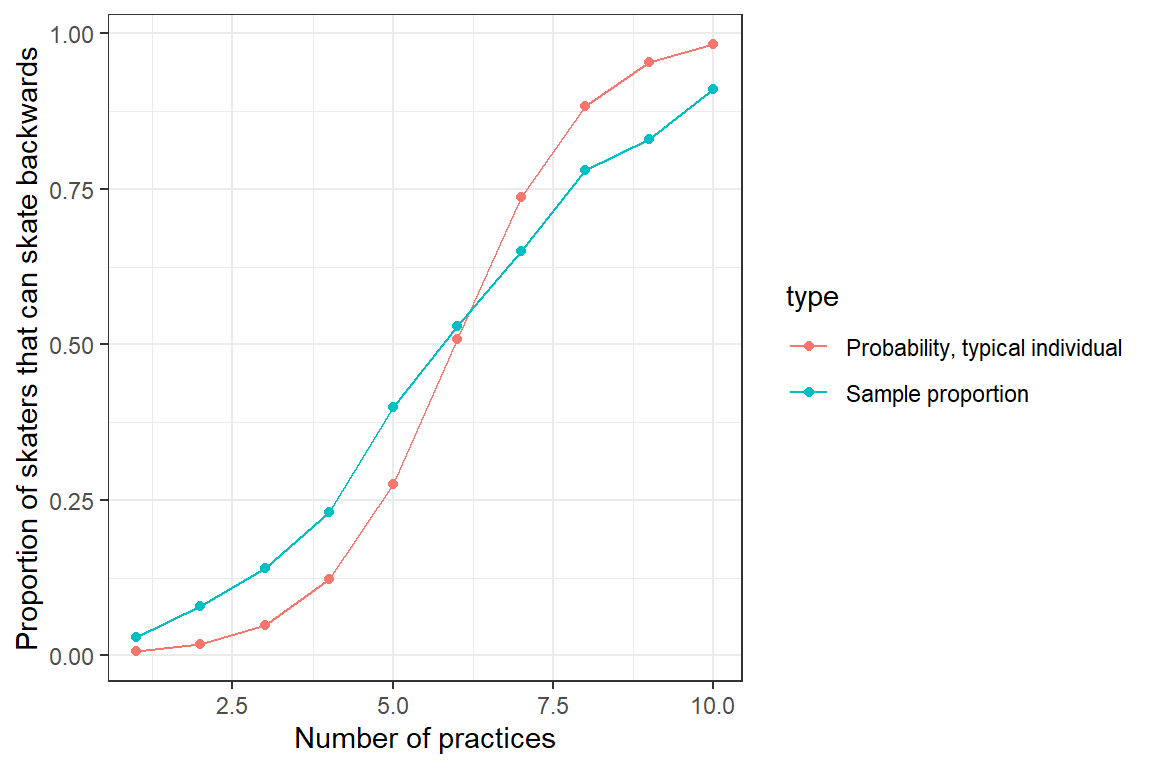
FIGURE 19.3: Sample proportion of skaters that can skate backwards as a function of the number of practices they have attended. Also plotted is the response curve for a typical individual with \(b_{0i} = 0\).
We see that the two curves do not line up – the predicted probability of skating backwards for a “typical individual” (with \(b_{0i} = 0\)) differs from the proportion of the sample that can skate backwards. This occurs because of the non-linear logit transformation, \(E[Y | X] \ne E[Y | X, b_{0i} = 0]\). To understand this mismatch, we next compare:
- the mean response curve for each individual on both the logit and probability scales
- the mean of these individual-specific curves on both the logit and probability scales
- the overall mean population response curve on both the logit and probability scales
We begin by computing the individual-specific curves, below:
pdat <- NULL
for (i in 1:nindividuals) {
  logitp.indiv <- beta_0 + b0_i[i] + practice.num * beta_1 # individual i's curve on logit scale
  p.indiv <- plogis(logitp.indiv) # individual i's curve on the probability scale
  tempdata <- data.frame(p = p.indiv,
                         logitp = logitp.indiv,
                         individual = i)
  pdat <- rbind(pdat, tempdata)
}
pdat$practice.num<-practice.num
We then calculate the average of the individual-specific curves on both the logit and probability scales:
pop.patterns<-pdat %>% group_by(practice.num) %>%
  dplyr::summarize(meanlogitp=mean(logitp), meanp=mean(p))
Lastly, we compare the individual-specific (i.e., subject-specific or conditional means; in black) to their average (in red) and to the population-average response curves (in blue) on both logit and probability response scales (Figure 19.4).
m1 <- ggplot(pdat, aes(practice.num, logitp)) +
  geom_line(aes(group = individual)) + ylab("logit p") +
  geom_line(data = pop.patterns, aes(practice.num, meanlogitp), col = "blue", linewidth = 1.2) +
  geom_line(data = mod, aes(practice.num, glmer.logit), col = "red", linewidth = 1.2, linetype = "dashed") +
  theme(legend.position = 'none') + xlab("Practice Number") +
  ylab(expression(Logit(p))) + ggtitle("A)")

m2 <- ggplot(pdat, aes(practice.num, p)) +
  geom_line(aes(group = individual)) + ylab("p") +
  geom_line(data = pop.patterns, aes(practice.num, meanp), col = "blue", size = 1.2) +
  geom_line(data = mod, aes(practice.num, glmer.p), col = "red", linewidth = 1.2, linetype = "dashed") +
  theme(legend.position = 'none') + xlab("Practice Number") +
  ylab(expression(p[i])) + ggtitle("B)")
## Warning: Using `size` aesthetic for lines was deprecated in ggplot2 3.4.0.
## ℹ Please use `linewidth` instead.
## This warning is displayed once every 8 hours.
## Call `lifecycle::last_lifecycle_warnings()` to see where this warning was generated.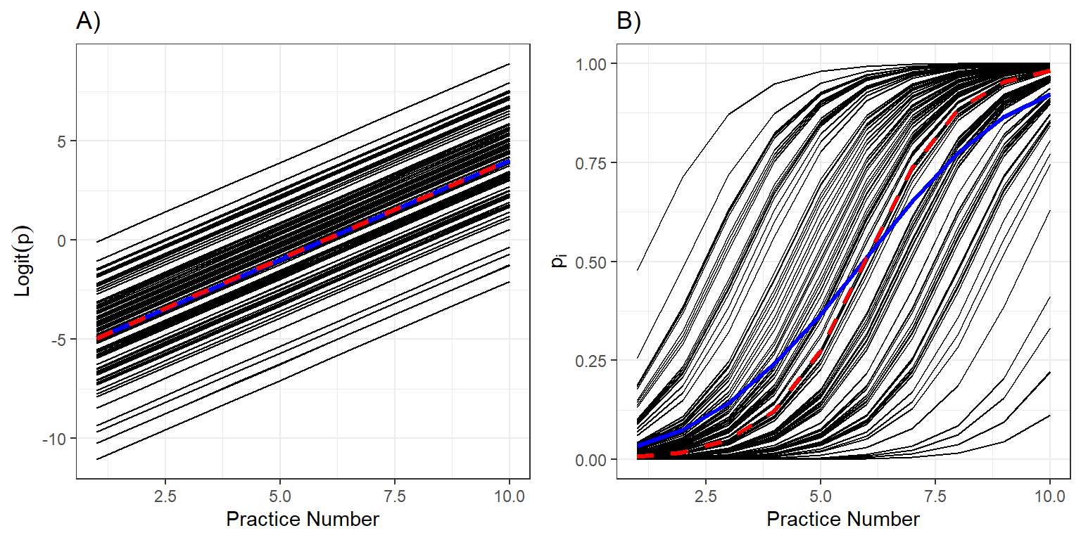
FIGURE 19.4: Individual response curves (black), the response curve for a typical individual with \(b_{0i} = 0\) (red), and the population mean response curve (blue) and on the logit and probability scales.
Let’s begin by looking at the predicted curves on the logit scale (Figure 19.4A). As expected, the logit probabilities of skating backwards increase linearly with the number of practices. Further, when we average the individual curves on the logit scale, we find that average of the individual-specific curves (in blue) and the curve for a typical individual with \(b_{0i}=0\) (in red) are identical (Figure 19.4A).
Now, let’s look at the same curves but on the probability scale (Figure 19.4B). We see that all individuals improve at the same rate (governed by \(\beta_1\)), but that they have different initial abilities (determined by \(b_{0i}\)). Thus, some individuals are able to skate backwards successfully by the 5th practice while others still have a low probability of skating backwards after 10 practices (Figure 19.4B). The average skater (with \(b_{0i} = 0\)), plotted in red, is extremely unlikely to skate backwards successfully after the first practice, but is nearly guaranteed to be skating backwards by the end of the season. When we average these curves, we find that there is a small, but non-negligible proportion of skaters that can skate backwards after the first practice and similarly, a small and non-negligible proportion of skaters that cannot skate backwards after 10 practices. The population mean curve (in blue) is flatter than the curve for a typical individual (in red). This will always be the case when fitting a logistic regression model with a random intercept – the population mean response curve will be attenuated with slope that is smaller in absolute value than the curve formed by setting all random effects equal to 0 (Zeger, Liang, & Albert, 1988; Fieberg et al., 2009).
If we are interested in directly modeling how the population mean (or proportion)82 changes as a function of one or more variables, we can consider Generalized Estimating Equations (Chapter 20). Alternatively, we can use the methods in the next section to approximate population mean response curves from fitted GLMMs.
19.8.1 Approximating marginal (population-average) means from fitted GLMMs
As discussed in Section 19.7, to calculate the marginal distribution (and thus, likelihood) of the data, we have to integrate over the distribution of the random effects. Unfortunately, there will not typically be a closed form solution to the integral that allows us to derive an analytical expression for the marginal distribution. Similarly, we will need to integrate over the distribution of the random effects to determine the marginal mean, \(E[Y|X] = \sum_y yf_{Y,b}(y) = \sum_y y \int f_{Y|b}(y)f_b(b)db\). Except for a few special cases (see Section 19.8.2), there will not generally be a closed form solution for this expression. Thus, we must resort to the same set of approaches discussed in Section 19.7 to derive an expression for the marginal mean. Specifically, we can:
- Approximate the integrand, \(\int f_{Y|b}(y)f_b(b)db\), in a way that gives us a closed form or known solution.
- Use numerical integration techniques to solve the integral.
- Use simulation techniques to approximate the solution to the integral.
19.8.2 Special cases
There are a few special cases where we can derive expressions for the marginal (population) means from the subject-specific parameters estimated when fitting generalized linear mixed effects models (Ritz & Spiegelman, 2004). We list a few of the more notable cases here. We already highlighted that setting \(b_{0i} = 0\) in linear mixed effects models will give us an expression for the marginal (population-average) mean (Section 19.3.1); this equivalence holds more generally for models with an identity link. Another important example is the case where a random intercept is added to a Poisson regression model:
\[\begin{gather} Y_{ij} |b_{0i} \sim Poisson(\lambda_{ij}) \nonumber \\ \log(\lambda_{ij}) = X_{ij}\beta+ b_{0i} \nonumber \\ b_{0i} \sim N(0, \sigma_{b_0}) \nonumber \end{gather}\]
In this case, the population-averaged response pattern is determined by adjusting the intercept: \(\beta^M_{0} = \beta^C_{0} + \sigma_{b_0}^2/2\), where \(\beta^M_{0}\) and \(\beta^C_{0}\) are the intercepts in the expression for the marginal and conditional means, respectively, and \(\sigma_{b_0}^2\) is the variance of the random intercept. The slope parameters will not need adjusting and have both conditional (subject-specific) and marginal (population-averaged) interpretations. We can demonstrate this result with another simple simulation example, below.
Assume 100 students in an ornithology class from the University of Minnesota go birding 20 times during the course of the semester. Each time out, they look for birds for between 30 min and 2 hours, recording the time they spent surveying to the nearest 5 minutes. Let \(Y_{ij}\) = the number of birds seen by student \(i\) during the \(j^{th}\) observation period and \(X_{ij}\) be the time (in hours) they spent looking for birds during the \(j^{th}\) observation period. Individuals will have different skill levels, which we represent using a Normally distributed random intercept, \(b_{0i}\). We will assume, conditional on \(b_{0i}\), that the number of birds observed can be described by a Poisson distribution with mean depending on the log number of hours of observation. Thus, we simulate data from the following model:
\[\begin{gather} Y_{ij} |b_{0i} \sim Poisson(\lambda_{ij}) \nonumber \\ \log(\lambda_{ij}) = \beta_0 + b_{0i} + \log(X_{ij})\beta_1 \nonumber \\ b_{0i} \sim N(0, \sigma_{b_0}), \nonumber \end{gather}\]
with parameters:
- \(\beta_0 = - 1.5\)
- \(\beta_1 = 0.2\)
- \(\sigma_{b_{0}} = 1.5\)
# Simulation set up
# Generate 100 random intercepts
set.seed(610)

# Sample size
nindividuals <- 100 # number of individuals
nperindivid <- 10 # number of observations per individual
ntotal <- nindividuals * nperindivid # total number of observations

# Data generating parameters
b0_i <- rnorm(nindividuals, 0, 1.5) # deviations from mean intercept
beta_0 <- -1.5 # mean intercept
beta_1 <- 0.2 # slope for time

# Generate 10 different observations for each individual Here, x will
# record the observation time to the nearest 5 minutes
lobs.time <- log(sample(seq(30, 120, by = 5), size = ntotal, replace = TRUE))

# Y|boi is Poisson lambda[ij]
loglam <- beta_0 + rep(b0_i, each = nperindivid) + lobs.time * beta_1
lam <- exp(loglam)
Y <- rpois(ntotal, lam)

# Create data set for model fitting
individual <- rep(1:nindividuals, each = nperindivid) # Cluster id
birdobs <- data.frame(Y = Y, lobs.time = lobs.time, individual = individual)
We then fit the GLMM corresponding to the data generating model and show that we are able to recover the parameter values used to simulate the data.
# ## Fit glmer model
# Estimates are close to values used to simulate data
fitsim <- glmer(Y ~ lobs.time + (1 | individual), family = poisson(), data = birdobs)
summary(fitsim)
## Generalized linear mixed model fit by maximum likelihood (Laplace Approximation) ['glmerMod']
## Family: poisson ( log )
## Formula: Y ~ lobs.time + (1 | individual)
## Data: birdobs
##
## AIC BIC logLik deviance df.resid
## 2382.9 2397.6 -1188.4 2376.9 997
##
## Scaled residuals:
## Min 1Q Median 3Q Max
## -2.4449 -0.5947 -0.3465 0.3592 4.5086
##
## Random effects:
## Groups Name Variance Std.Dev.
## individual (Intercept) 1.924 1.387
## Number of obs: 1000, groups: individual, 100
##
## Fixed effects:
## Estimate Std. Error z value Pr(>|z|)
## (Intercept) -1.95290 0.33671 -5.800 6.63e-09 ***
## lobs.time 0.31214 0.07018 4.448 8.68e-06 ***
## ---
## Signif. codes: 0 '***' 0.001 '**' 0.01 '*' 0.05 '.' 0.1 ' ' 1
##
## Correlation of Fixed Effects:
## (Intr)
## lobs.time -0.895## Computing profile confidence intervals ...## 2.5 % 97.5 % trueparam
## .sig01 1.1759471 1.6614586 1.5
## (Intercept) -2.6309957 -1.2907895 -1.5
## lobs.time 0.1733807 0.4525831 0.2Next, we compute and plot the following:
- the estimated mean response curve for a typical student, \(E[Y_{ij} | X_{ij}, b_{0i} = 0] = \exp(\beta_0 + \beta_1 \log(X_{ij}))\)
- the estimated mean response curve for the population of students, \(E[Y_{ij} | X_{ij}] = \exp(\beta_0 + \sigma^2_{b_0}/2 + \beta_1 \log(X_{ij}))\)
- the mean number of birds observed in the population of students as a function of log(observation time)
# Summarize the mean number of birds seen as a function of lobs.time at the population-level
mdatb <- birdobs %>% group_by(lobs.time) %>% dplyr::summarize(meanY = mean(Y))

# Now, add on appropriate conditional and population average mean
# response curves
mdatb$ss <- exp(fixef(fitsim)[1] + mdatb$lobs.time * fixef(fitsim)[2])
mdatb$pa <- exp(fixef(fitsim)[1] + as.data.frame(VarCorr(fitsim))[1,4] / 2 +
                 mdatb$lobs.time * fixef(fitsim)[2])

# plot
ggplot(mdatb, aes(lobs.time, meanY)) + geom_point() +
  geom_line(aes(lobs.time, ss), color="red") +
  geom_line(aes(lobs.time, pa), color="blue") +
  xlab("log(Observation time)") + ylab("Number of birds seen")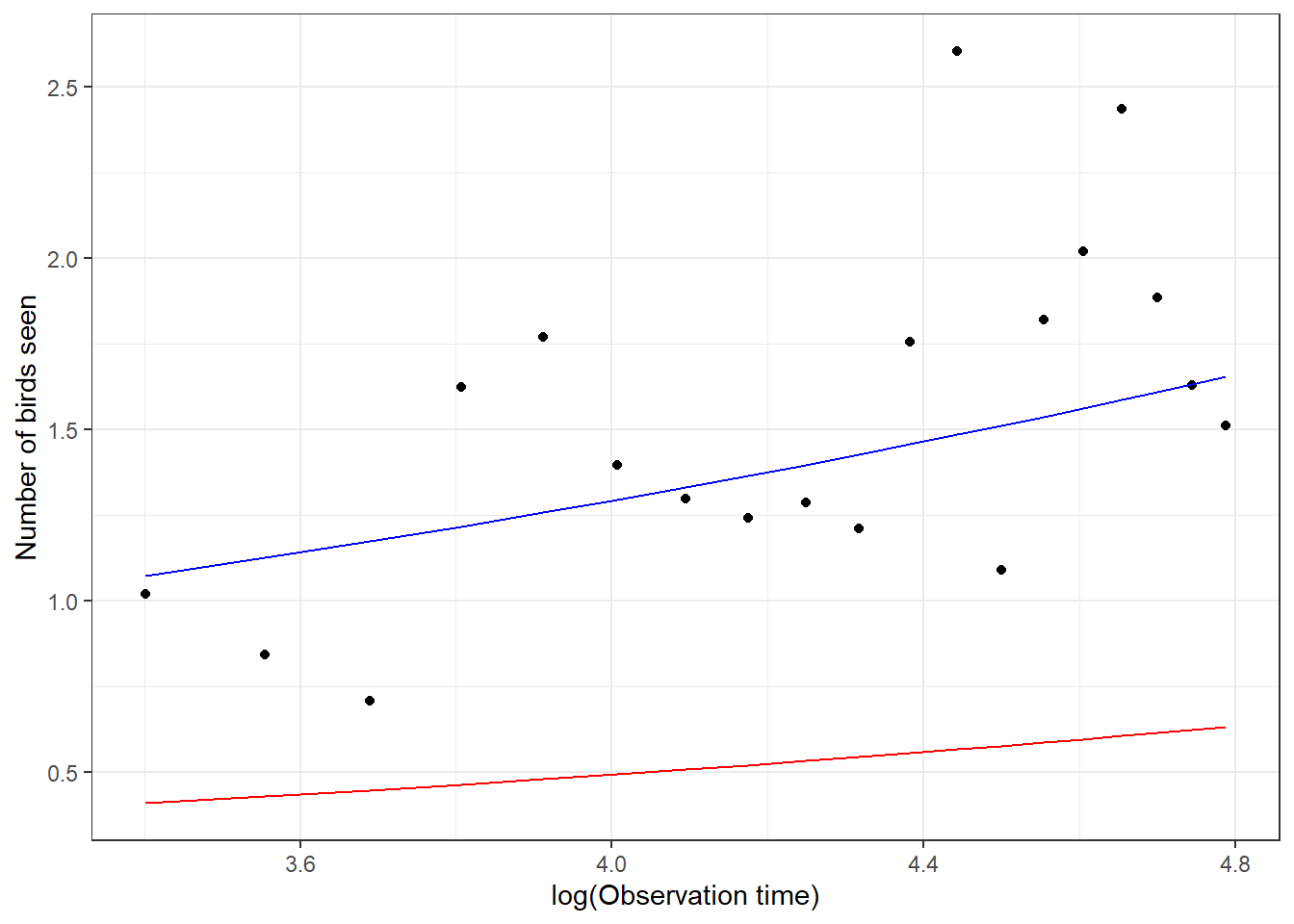
FIGURE 19.5: Comparison of the mean response curve for a typical student (red), formed by setting \(b_{0i} = 0\), estimated from a Poisson generalized linear mixed effects model (GLMM) with the mean response curve for the population of students (blue) estimated by adjusting the intercept from the fitted GLMM. Points represent the empirical means at each log(observation) time.
Examining Figure 19.5, we see that the mean response curve for the “typical student”, formed by setting \(b_{0i} = 0\) (in red) underestimates the number of birds seen in the population of students. However, the mean response curve derived by adjusting the intercept (blue curve) fits the data well. This adjustment is only appropriate when fitting Poisson GLMMs that include only a random intercept but no random slope terms.
Another important case where we can derive expressions for the marginal mean from a fitted random-effects model is when using Probit regression (eq. (19.9); Ritz & Spiegelman, 2004; Young, Preisser, Qaqish, & Wolfson, 2007):
\[\begin{gather} Y_{ij} | b_{0i} \sim Bernoulli(p_i) \nonumber \\ p_i = \Phi(X_{ij}\beta + b_{0i}), \tag{19.9} \end{gather}\]
where \(\Phi\) is the cumulative distribution function of the standard Normal distribution (and can be calculated using the pnorm function in R). In this case, marginal parameters, \(\beta_M\) can be derived from conditional parameters \(\beta_C\) and the random effects variance component, \(\sigma^2_{b_0}\) using:
\[\beta^M = \frac{\beta^C}{\sqrt{\sigma^2_{b_0} +1}}\]
Lastly, we note that Zeger et al. (1988) derived a useful approximation for describing marginal (i.e., population average) mean response patterns using the parameters estimated from a generalized linear mixed effects model in the case of logistic regression with a random intercept:
\[\begin{equation} \beta^M = (\sigma^2_{b_0}0.346 +1)^{-1/2}\beta^C \tag{19.10} \end{equation}\]
This approximation works well for our simulated hockey player data (Figure 19.6).
sigma2b0 <- as.data.frame(VarCorr(glmermod))[1, 4]
betaM_0 <- fixef(glmermod)[1]/sqrt(sigma2b0 * 0.346 +1)
betaM_1 <- fixef(glmermod)[2]/sqrt(sigma2b0 * 0.346 +1)
mdat3<-rbind(mdat2,
             data.frame(practice.num = practice.num,
                        p = plogis(betaM_0 + betaM_1 * practice.num),
                        type = rep("Zeger approximation", 10)))

# Plot
ggplot(mdat3, aes(practice.num, p, col=type)) +
  geom_line() + geom_point() +
  xlab("Number of practices") +
  ylab("Proportion of skaters that can skate backwards")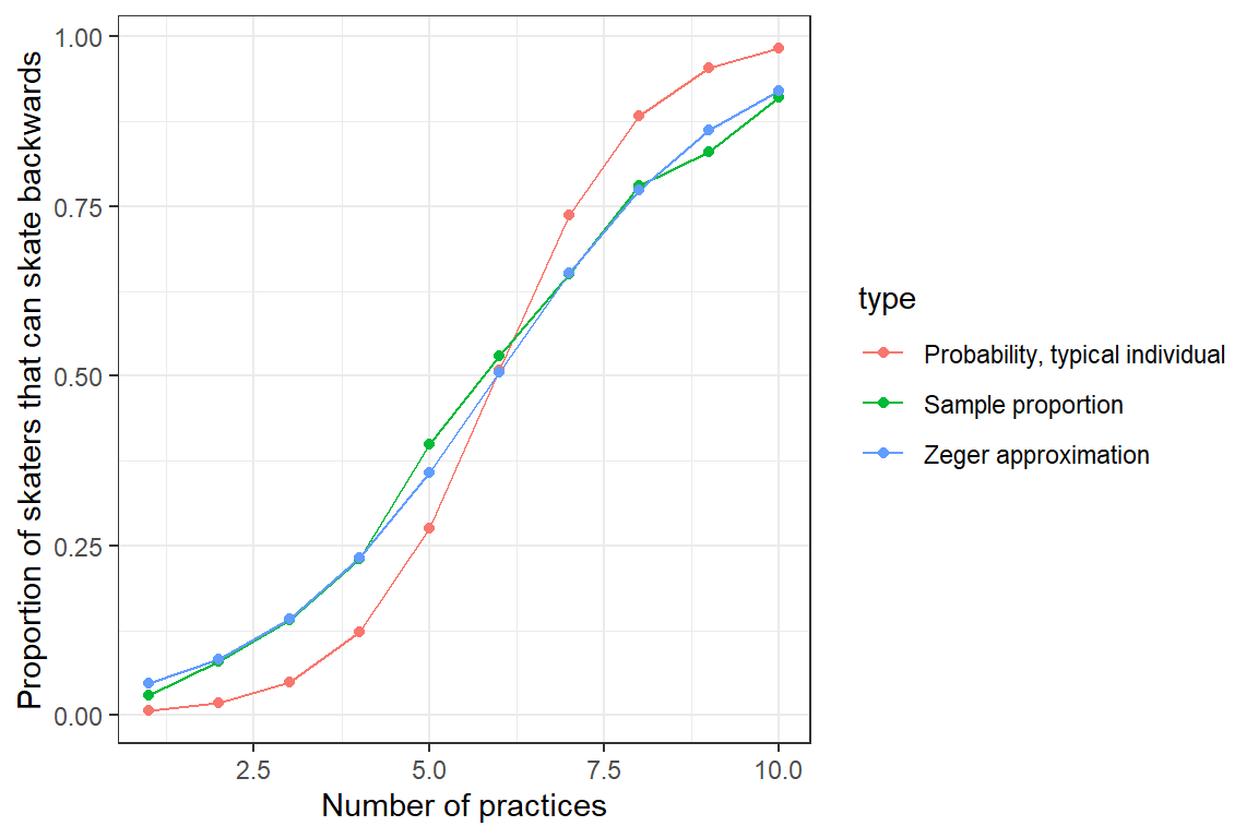
FIGURE 19.6: Population mean response curve using Zeger’s approximation (eq. (19.10); blue) versus the response curve for a typical individual formed by setting \(b_{0i} = 0\) (green). Population proportions are indicated by the red curve.
Again, this approximation only works for logistic regression models containing random intercepts but not random slopes. Alternatively, we can use numerical integration to average over the distribution of the random effects and thereby determine the marginal mean response curve.
19.8.3 Numerical integration
Recall, to determine the marginal mean response curve, we need to integrate over the distribution of the random effects:
\[\begin{equation} E[Y|X] = \sum_y y f_{Y,b}(y) = \sum_Y y\int f_{Y| b}(y)f_b(b)db \tag{19.11} \end{equation}\]
For binary regression models, note that \(Y\) can take only 1 of 2 values (0 and 1), and only the value of 1 contributes a term to the expected value (eq. (19.11)). Furthermore, when \(Y =1\), \(f_{Y|b}(y) = \frac{e^{\beta_0 + b + \beta_1 X}}{1 + e^{\beta_0 + b + \beta_1 X}}\). Lastly, \(f_b(b)\) is a Normal distribution with mean 0 and variance \(\sigma^2_{b_0}\). Thus, we need to compute:
\[E[Y|X] = \sum_y yf_{Y,b}(y) =\int \frac{e^{\beta_0 + b + \beta_1 X}}{1 + e^{\beta_0 + b + \beta_1 X}}\frac{1}{\sqrt{2 \pi}\sigma}e^{-\frac{b^2}{2\sigma^2_{b_0}}}db\]
We could make use of the integrate function in R to approximate this integral, as we demonstrate below for our model describing how quickly young hockey players learn how to skate backwards. We then plot the result (Figure 19.7).
# Matrix to hold marginal mean response curve, E[Y|X]
pa.rate<-matrix(NA,10,1)
  for(i in 1:10){
     intfun<-function(x){
       plogis(fixef(glmermod)[1] + x + practice.num[i]*fixef(glmermod)[2])*dnorm(x,0,sqrt(sigma2b0))}
       pa.rate[i]<-integrate(intfun,-Inf, Inf)[1]
   }
mdat4<-rbind(mdat2,
             data.frame(practice.num = practice.num,
                        p = unlist(pa.rate),
                        type = rep("Marginal mean by Integration", 10)))

# Plot
ggplot(mdat4, aes(practice.num, p, col=type)) +
  geom_line() + geom_point() +
  xlab("Number of practices") +
  ylab("Proportion of skaters that can skate backwards")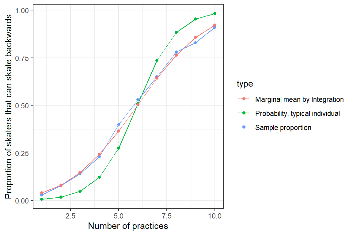
FIGURE 19.7: Population mean response curve determined by numerical integration (red) versus the response curve for a typical individual, formed by setting \(b_{0i} = 0\) (green). Population proportions are indicated by the blue curve.
Again, we see that we are able to approximate the population proportions well once we translate the fit of our GLMM to a prediction about the marginal mean response curve.
19.8.4 Simulation
Rather than use numerical integration, we could solve for marginal response patterns using a simulation approach, where we:
- generate a large sample of random effects from the fitted random-effects distribution, \(N(0, \hat{\sigma}^2_{b_0})\);
- generate the conditional, subject-specific curves for each of these randomly chosen individuals;
- average the subject-specific curves from step 2 to estimate the marginal mean response curve.
We leave this as a potential exercise.
19.8.5 Approximating marginal means using GLMMadpative
In Sections 19.8.3 and 19.8.4, we discussed approaches for piecing together marginal response curves that essentially estimate \(E[Y_i | X_i]\) at a set of unique values of \(X_i\) chosen by the user. We can then plot \(E[Y_i | X_i]\) versus \(X_i\) to examine these marginal (population-average) response curves. However, these approaches do not give us a set of marginal coefficients for summarizing the effects of \(X_i\) at the population level. In Section 19.8.2, we saw a few special cases where we could derive or approximate marginal or population-level regression parameters from the fitted GLMM. In this section, we will explore the GLMMadaptive package (Rizopoulos, 2021), which provides a function, marginal_coefs, that estimates coefficients describing marginal response patterns for a wider variety of GLMMS.
We begin by fitting the same GLMM to our simulated skating data, but using the mixed_model function in the GLMMadaptive package. Its syntax is similar to that of lme in the nlme package:
library(GLMMadaptive)
fit.glmm <- mixed_model(fixed = Y ~ practice.num,
  random = ~ 1 | individual,
  family = binomial(link = "logit"),
  data = skatedat
)
summary(fit.glmm)
##
## Call:
## mixed_model(fixed = Y ~ practice.num, random = ~1 | individual,
## data = skatedat, family = binomial(link = "logit"))
##
## Data Descriptives:
## Number of Observations: 1000
## Number of Groups: 100
##
## Model:
## family: binomial
## link: logit
##
## Fit statistics:
## log.Lik AIC BIC
## -379.886 765.772 773.5875
##
## Random effects covariance matrix:
## StdDev
## (Intercept) 2.230948
##
## Fixed effects:
## Estimate Std.Err z-value p-value
## (Intercept) -5.9444 0.4860 -12.2303 < 1e-04
## practice.num 0.9960 0.0709 14.0464 < 1e-04
##
## Integration:
## method: adaptive Gauss-Hermite quadrature rule
## quadrature points: 11
##
## Optimization:
## method: hybrid EM and quasi-Newton
## converged: TRUEWe see that we get very similar answers as to when we fit the model using the glmer function. The mixed_model function uses numerical integration to approximate the likelihood (see Section 19.7), but uses more quadrature points than glmer does by default, and thus, should result in a more accurate approximation of the likelihood. In addition, the glmer function only uses numerical integration when fitting models with a single random intercept, whereas the mixed_model function can perform numerical integration for models that include random intercepts and random slopes. Another advantage of mixed_model over glmer is that it can fit zero-inflated Poisson and Negative Binomial models that allow for random effects in the zero part of the model; glmmTMB also has this capability, but it only uses the Laplace approximation when fitting models (see Section 19.7). On the other hand, the mixed_model function only allows for a single grouping factor for the random effects whereas glmer and glmmTMB can fit models using multiple grouping factors (e.g., one could include (1 | individual) and (1 | year) for an analysis of data that included many individuals followed for many years).
The primary reason we will explore mixed_model in the GLMMadaptive package is because of its ability to provide coefficient estimates, \(\hat{\beta}^M\), for describing marginal response patterns. The marginal_coefs function estimates these coefficients via the following method (Hedeker, Toit, Demirtas, & Gibbons, 2018):
- Marginal means at the observed \(X_i\) are estimated using Monte Carlo simulations (Section 19.8.4). Specifically, a large number of random effects are generated from a Normal distribution, \(b^{sim} \sim N(0, \hat{\Sigma}_b)\). These simulated random effects are then used to estimate subject-specific means, \(\hat{E}[Y_i | X_i, b^{sim}]\). The subject-specific means are then averaged to form population-averaged means, \(\hat{E}[Y_i | X_i]\).
- Marginal coefficients, \(\beta^M\), are estimated by fitting a linear model with \(\text{logit}(\hat{E}[Y_i |X_i])\) as the response variable and \(X_i\) as the predictor variable. This results in the following estimator:
\[\begin{equation} \hat{\beta}^M = (X'X)^{-1}X' \text{logit}(\hat{E}[Y_i |X_i]), \tag{19.12} \end{equation}\]
Below, we calculate these marginal coefficients and compare them to our estimates using numerical integration, the estimated mean curve for a “typical skater” (formed by setting \(b_{0i}=0\)), and to the population proportions at each practice number (Figure 19.8).
marginal_beta <- marginal_coefs(fit.glmm, std_errors = FALSE)
mdat5<-rbind(mdat4,
             data.frame(practice.num = practice.num,
                        p = plogis(marginal_beta$betas[1]+practice.num * marginal_beta$betas[2]),
                        type = rep("GLMMadaptive", 10)))

# Plot
ggplot(mdat5, aes(practice.num, p, col=type)) +
  geom_line() + geom_point() +
  xlab("Number of practices") +
  ylab("Proportion of skaters that can skate backwards")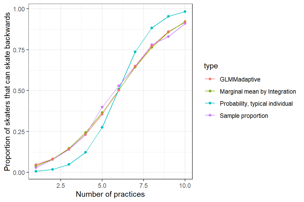
FIGURE 19.8: Population mean response curve determined by numerical integration (olive green) and using the marginal_coef function (red) from the GLMMadaptive package versus the response curve for a typical individual (formed by setting \(b_{0i} = 0\); aqua blue). Population proportions are given in purple.
Again, we see that we are able to recover marginal (population-average) response patterns using this approach, but with the advantage of being able to report population-level odds ratios:
## practice.num
##     1.830493
I.e., we can report that the odds of skating backwards increases by a factor of 1.8 at the population level for each additional practice. This odds ratio will always be smaller than the corresponding subject-specific odds ratio that holds \(b_{0i}\) constant:
## practice.num
##     2.710188
Again, the difference is expected since the subject-specific curves rise faster than the population average curve (Figure 19.4B).
19.9 Hypothesis testing and modeling strategies
Methods for selecting an appropriate model and testing hypotheses involving regression parameters in generalized linear mixed effects models typically rely on an asymptotic Normality assumption. Thus, we do not have to worry about various degrees-of-freedom approximations, and there is no REML option to consider. On the other hand, inference is more reliant on large samples. In addition, the challenges associated with fitting GLMMS (see Section 19.7) often limits the complexity of the models we can fit, particularly with binary data which tend to be less informative than continuous data (e.g., see Section 8.5).
Below, we reconsider our model for the mallard nest occupancy data and show how the Anova function can be used to test hypotheses regarding the fixed effects parameters:
## Analysis of Deviance Table (Type II Wald chisquare tests)
##
## Response: nest
##                    Chisq Df Pr(>Chisq)
## year              0.8804  2  0.6438999
## period            2.0199  3  0.5682928
## deply             0.0871  1  0.7678415
## vom               0.0028  1  0.9579025
## poly(wetsize, 2) 17.9392  2  0.0001272 ***
## year:period      13.3628  6  0.0376227 *
## period:vom       10.5617  3  0.0143483 *
## ---
## Signif. codes:  0 '***' 0.001 '**' 0.01 '*' 0.05 '.' 0.1 ' ' 1
Based on the significant interactions, it seems reasonable to stick with the full model for inference. We would conclude that nest occupancy rates depend on vom, but that the relationship between voc and nest occupancy varies by period. We might also consider using functions in the ggeffects package to explore the non-linear relationship between wetland size and nest occupancy (Figure 19.9).
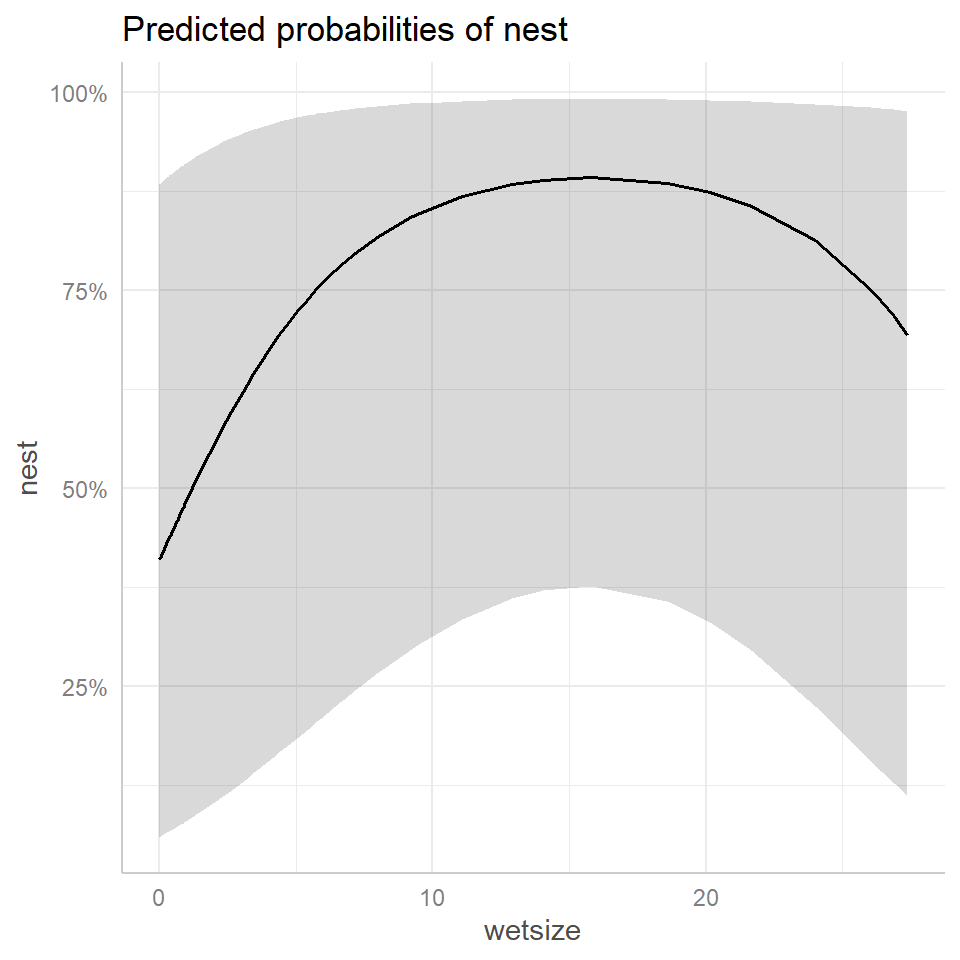
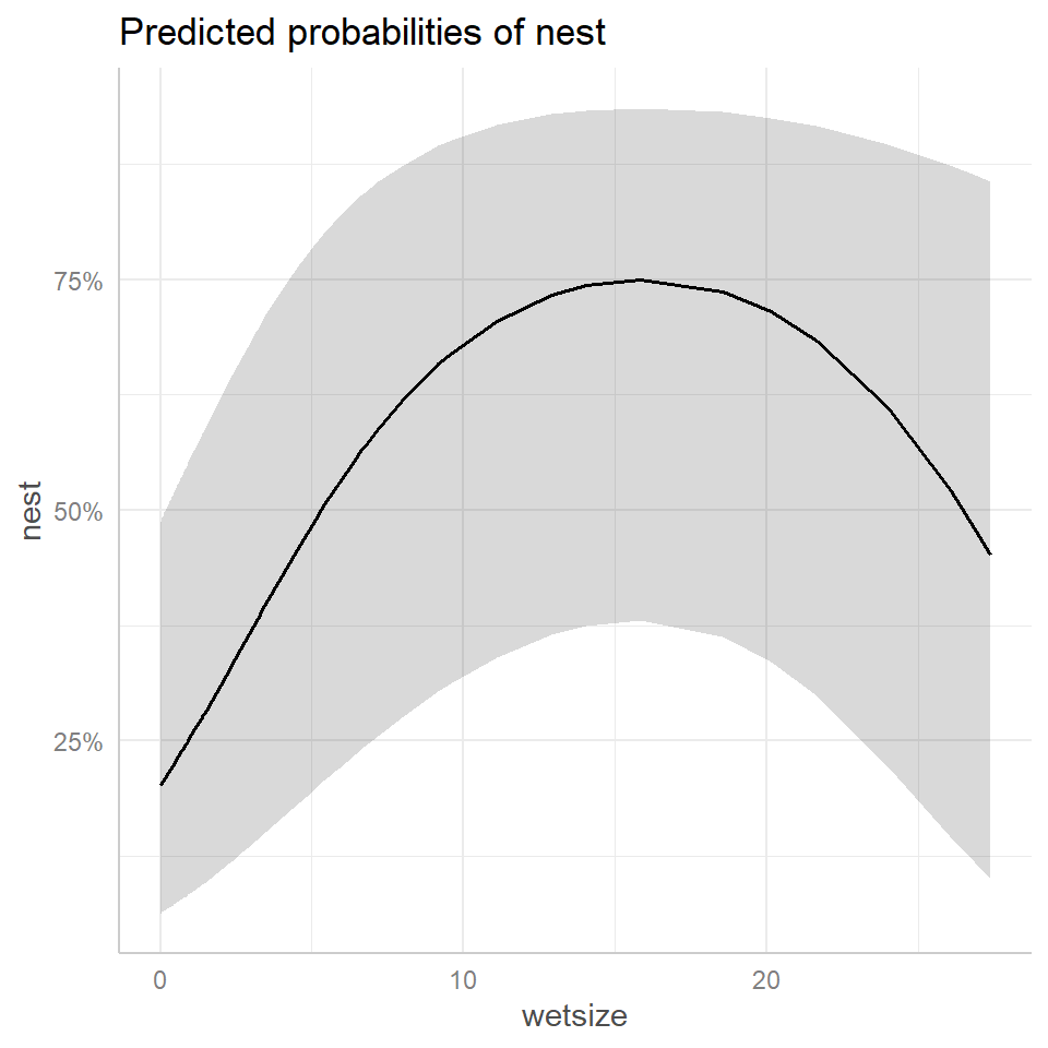
FIGURE 19.9: Effect plots using the ggpredict (left panel) and ggeffect (right panel) functions in the ggeffects package (Lüdecke, 2018) depicting the relationship between wetland size (wetsize) on nest occupancy rates inferred from the generalized linear mixed effects model fit to the data from Zicus, Rave, Das, et al. (2006).
To understand what is plotted, we can look at the output from the ggpredict and ggeffect functions.
## # Predicted probabilities of nest
##
## wetsize | Predicted |       95% CI
## ----------------------------------
##    0.00 |      0.41 | [0.06, 0.88]
##    0.23 |      0.43 | [0.06, 0.89]
##    0.63 |      0.46 | [0.07, 0.90]
##    1.37 |      0.51 | [0.09, 0.92]
##    3.14 |      0.63 | [0.13, 0.95]
##    5.05 |      0.72 | [0.19, 0.97]
##    7.19 |      0.80 | [0.25, 0.98]
##   27.39 |      0.69 | [0.11, 0.98]
##
## Adjusted for:
## *   year = 1997
## * period =    1
## *  deply =    1
## *    vom = 0.89
## * strtno = 0 (population-level)
##
## Not all rows are shown in the output. Use `print(..., n = Inf)` to show all rows.The output from ggpredict is relatively easy to understand – these are predictions formed by setting all covariates other than the focal covariate (wetsize) to specific values listed below the output. The random effect is also set to 0, implying that these are predictions for a “typical” subject when year = 1997, period = 1, deply = 1 (single cylinder), and vom = 0.89.
Now, let’s look at the output from ggeffect.
## # Predicted probabilities of nest
##
## wetsize | Predicted |       95% CI
## ----------------------------------
##    0.00 |      0.20 | [0.06, 0.49]
##    0.23 |      0.21 | [0.07, 0.50]
##    0.63 |      0.23 | [0.08, 0.53]
##    1.37 |      0.28 | [0.09, 0.58]
##    3.14 |      0.38 | [0.14, 0.69]
##    5.05 |      0.49 | [0.20, 0.79]
##    7.19 |      0.59 | [0.26, 0.86]
##   27.39 |      0.45 | [0.10, 0.86]
##
## Not all rows are shown in the output. Use `print(..., n = Inf)` to show all rows.The output from ggeffect is more difficult to decipher as it is averaging over the values of the other covariates in some way. I also suspect that it is setting the random effect to 0. We can see this if we compare our earlier plots for the ice skating example to the output from ggeffects (Figure 19.10). The response pattern from ggeffects most closely matches the response curve for a typical individual formed by setting the random effect equal to 0.
 ggplot(mdat2, aes(practice.num, p, col=type)) +
     geom_line() + geom_point() +
     xlab("Number of practices") +
     ylab("Proportion of skaters that can skate backwards") +
     theme(legend.position = "bottom", legend.box = "horizontal")
plot(ggeffect(glmermod)) 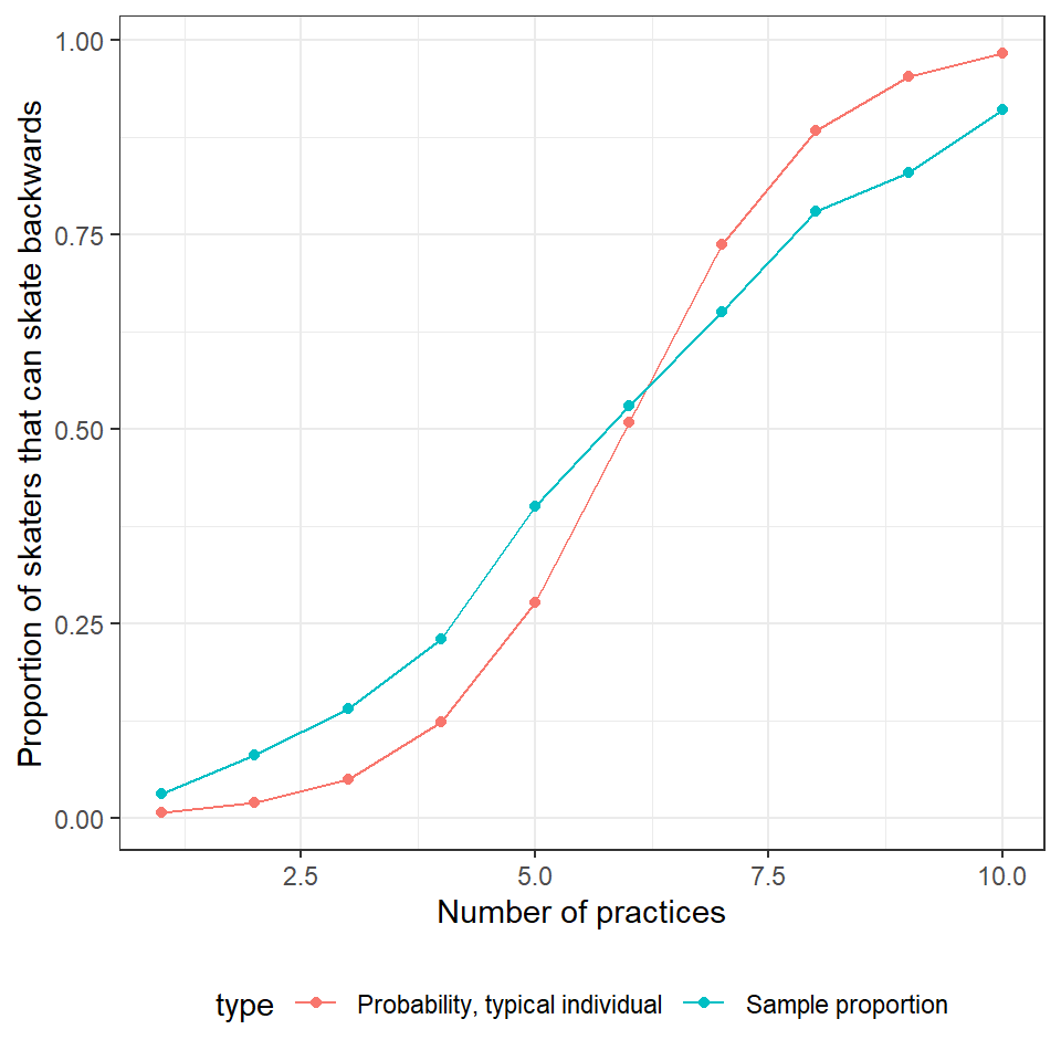
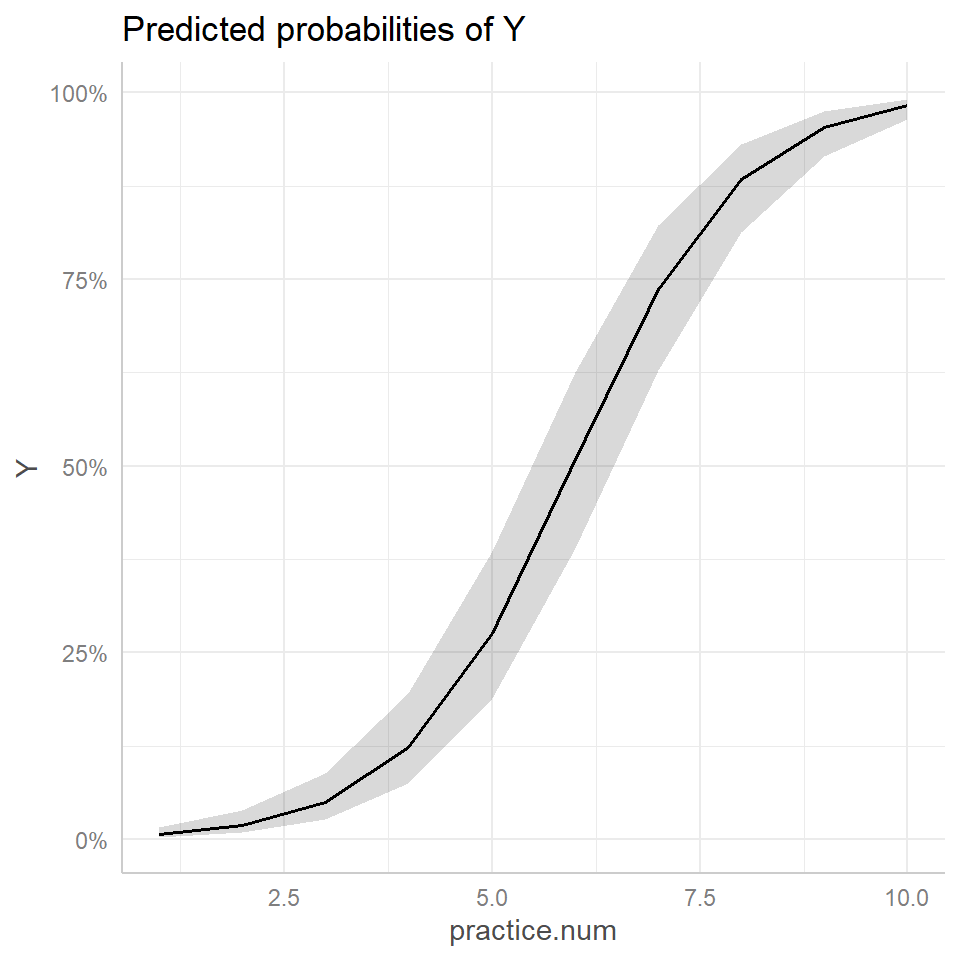
FIGURE 19.10: Comparison of effect plot created using the ggeffects function (right panel) to the response curve for a typical individual, formed by setting \(b_{0i} = 0\) (left panel, red). Population proportions are indicated by the aqua blue curve in the left panel.