This book is in Open Review. I want your feedback to make the book better for you and other readers. To add your annotation, select some text and then click the on the pop-up menu. To see the annotations of others, click the in the upper right hand corner of the page

Chapter 17 Models for zero-inflated data

Learning objectives

1. Be able to fit models to response data with lots of zeros (hurdle and zero-inflated models).

2. Be able to describe these models and their assumptions using equations and text and match parameters in these equations to estimates in computer output.

17.1 R packages

We begin by loading a few packages upfront:

set.seed(1288)
library(patchwork) # for creating multi-panel plots
library(ggplot2) # for plotting
library(R2jags) # for interfacing with JAGS
library(MCMCvis) # for summarizing MCMC output
library(mcmcplots) # for visualizing MCMC output
library(sjPlot) # for creating tables
library(modelsummary) # for creating tables 
library(dplyr) # for data wrangling
library(knitr) # for creating reproducible reports
library(MASS) # for fitting negative binomial regression models
library(pscl) # for fitting zero-inflated models

In addition, we will use data and functions from the following packages:

• Data4Ecologists for the slugs data set
• glmmTMB for fitting zero-inflated models

17.2 Zero-inflation

Presence-absence and count data collected in ecological monitoring efforts are often analyzed using models that allow for zero-inflation – i.e., an overabundance of 0’s. The first thing to note about zero-inflation is that it refers to response data, \(Y_i\), not predictors, \(X_i\). Although we will focus on zero-inflated count data, zero-inflation is also relevant to binary data (e.g., occupancy models as discussed in Chapter 20 of Kéry, 2010), and continuous data (e.g., Friederichs, Zimmer, Herwig, Hanson, & Fieberg, 2011).

There are many reasons why we may end up with an overabundance of zero counts in ecological monitoring data sets:

• sites may not be suitable for the species;
• the species may occur at low densities, and therefore suitable sites may not all be occupied;
• our sampling effort may not have been sufficient to detect individuals that use the site or we may have sampled during times when individuals are difficult to detect;
• we may have mistaken individuals for the wrong species.

Common statistical distributions used to model count data, including the Poisson and Negative Binomial distributions, allow for zeros:

• Poisson Distribution: \(P(Y_i = 0) = \exp(-\lambda_i)\)
• Negative Binomial Distribution: \(P(Y_i = 0) = \Big(\frac{\theta}{\mu+\theta}\Big)^\theta\)

Zero-inflation refers to situations where there are more zeros than expected given the assumed statistical distribution. In regression applications, we are allowing the mean of these distributions to depend on predictor variables. There may be some regions of “predictor space” where the mean is really small, and thus, where we might expect to find many zeros. So, a lot of zeros does not necessarily mean that data are zero-inflated. As the mean gets larger, however, we should expect fewer zeros. When certain regions of predictor space have both a large mean and many zeros, we might want to consider models that allow for zero-inflation.

17.3 Testing for excess zeros

How can we determine if we have excess zeros (i.e., zero-inflated data)? One option would be to modify our goodness-of-fit test (see Section 15.4.5) to use the number of zeros in our data set as the test statistic (rather than the sum of Pearson residuals). To demonstrate, let’s revisit the slug data from Sections 10 and 15.

library(Data4Ecologists)
data(slugs) 

We will use the total number of zeros as our test statistic: \(T = \sum_{i=1}^n I(Y_i=0)\). Let’s work through the different steps involved in the hypothesis test:

1. State null and alternative hypotheses,

• \(H_0:\) the data are consistent with a Poisson
• \(H_A:\) the data are not consistent with a model with separate \(\lambda\)s for the field and Rookery sites; there are more 0’s than expected if the data followed separate Poisson distributions for each site.

2. Calculate a statistic that measures the discrepancy between the data and the null hypothesis. Here, we will use \(T =\) the number of zeros in the data set.

3. Determine the distribution of the statistic in step 2 when the null hypothesis is true. We will determine the distribution of \(T\) when the null hypothesis is true using simulations, allowing for uncertainty in our values of \(\lambda_i\).

4. Compare the statistic for the observed data [step 2] to the distribution of the statistic when the null hypothesis is true [step 3]. The p-value = the probability of getting a value of \(T\) as big or bigger than the value for our observed data.

# Fitted model
  fit.pois<-glm(slugs~field, data=slugs, family=poisson())

 # Number of simulations
  nsims<-10000

# Set up matrix to hold goodness-of-fit statistics
  zeros.sim<-matrix(NA, nsims, 1)
  nobs<-nrow(slugs) # number of observations
  
# Extract the estimated coefficients and their asymptotic variance/covariance matrix  
# Use these values to generate nsims new betas (beta.hat)  
  beta.hat<-MASS::mvrnorm(nsims, coef(fit.pois), vcov(fit.pois))

# Design matrix for creating new lambda^'s    
  xmat<-model.matrix(fit.pois)
  for(i in 1:nsims){
    # Generate lambda^'s    
    lambda.hat<-exp(xmat%*%beta.hat[i,])
    # Generate new simulated values
    new.y<-rpois(nobs, lambda = lambda.hat)
    # Count the number of zeros
    zeros.sim[i]<-sum(new.y==0)
  }

We can then plot the distribution of \(T\) when the null hypothesis is true and overlay the number of zeros from our actual data set (Figure 17.1).

# T for our data
(T<-sum(slugs$slugs==0))

## [1] 34

hist(zeros.sim, xlab="# of zeros", ylab="Density", main="", col="gray", xlim=c(0, 35))
abline(v = T, col = "blue")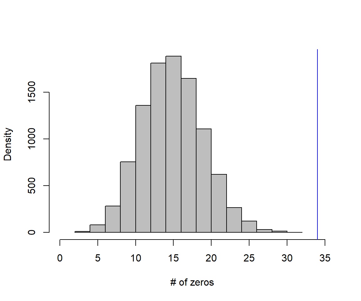

FIGURE 17.1: Distribution of zeros in data sets generated by the assumed Poisson regression model. Note that our test statistic (number of zeros in our original data set, which equaled 34) falls way out in the tail of the distribution, giving us a p-value of essentially 0.

Lastly, we calculate the p-value as the probability of getting a value of \(T \ge 34\) when the null hypothesis is true:

#pvalue
sum(zeros.sim>=T)/nsims

## [1] 0

Clearly, there are more zeros in the observed data than one might expect if the data were Poisson distributed with separate \(\lambda\)s for each site.

17.4 Zeros and the Negative Binomial model

Before considering zero-inflated models, it is important to recognize that the Negative Binomial distribution often provides a reasonable fit to data with many zeros. This has been my experience, and is also the view that has been expressed by Paul Allison, a statistician with lots of experience analyzing real data - see his blog here.

For example, if we repeat the goodness-of-fit test from the last section with a negative binomial model, we find that we do not reject the null hypothesis (Figure 17.2).

# Fitted model
  fit.nb<-MASS::glm.nb(slugs~field, data=slugs)

 # Number of simulations
  nsims<-10000

# Set up matrix to hold goodness-of-fit statistics
  zeros.sim<-matrix(NA, nsims, 1)
  nobs<-nrow(slugs) # number of observations
  
# Extract the estimated coefficients and their asymptotic variance/covariance matrix  
# Use these values to generate nsims new beta's  
  beta.hat<-MASS::mvrnorm(nsims, coef(fit.nb), vcov(fit.nb))
  theta.hat<-rnorm(nsims, fit.nb$theta, fit.nb$SE.theta)
      
# Design matrix for creating new lambda^'s    
  xmat<-model.matrix(fit.nb)
  for(i in 1:nsims){

    # Generate lambda^'s and thetas    
    mus<-exp(xmat%*%beta.hat[i,])
    
    # Generate new simulated values
    new.y<-rnbinom(nobs, mu = mus, size=theta.hat[i])

    # Count the number of zeros
    zeros.sim[i]<-sum(new.y==0)
  }

Warning in rnbinom(nobs, mu = mus, size = theta.hat[i]): NAs produced

# T for our data
hist(zeros.sim, xlab="# of zeros", ylab="Density", main="", col="gray")
abline(v = T, col = "blue")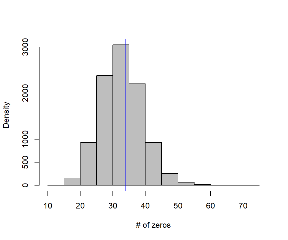

FIGURE 17.2: Distribution of zeros in data sets generated by the assumed negative binomial regression model. In this case, our test statistic (T = 34) falls near the mean of the distribution, and we fail to reject the null hypothesis that the data are consistent with the Negative Binomial regression model.

#pvalue
ind<-is.na(zeros.sim)!=TRUE # some NAs due to getting negative thetas
sum(zeros.sim[ind]>=T)/sum(ind)

[1] 0.4681468

17.5 Hurdle models

There are two general classes for modeling zero-inflated data, Hurdle models and zero-inflated mixture models. We will briefly introduce hurdle models here but then focus on the latter class of model for the rest of this section. Hurdle models contain two different sub-components:

1. A model for whether or not an observation is 0.
2. A truncated count model for the non-zero observations.

These models can be fit using a two-step approach:

1. Create a data set with new response variable, \(Z_i\), indicating whether the original response is a 0 or not:

\[Z_{i} = \left\{ \begin{array}{ll} 1 & \mbox{if } Y_i = 0\\ 0 & \mbox{if } Y_i \ne 0 \end{array} \right.\]

Model \(Z_i\) using logistic regression:

\[\begin{equation} \begin{split} Z_i \sim Bernoulli(p_i) \\ logit(p_i) = \beta_0 + \beta_1X_{i,1}+\ldots \beta_pX_{i,p} \end{split} \tag{17.1} \end{equation}\]

2. Create a second data set containing only the non-zero observations, \(\widetilde{Y}_i\). Model \(\widetilde{Y}_i\) using a truncated count distribution, usually either a truncated-Poisson or truncated Negative Binomial. A truncated distribution is one in which we modify the probability mass function to exclude values below a threshold (in this case we exclude the possibility of a zero; see Section 17.5.1).

Alternatively, hurdle models can be fit in one step using the zeroinfl function in the pscl library. Fitting the model in a single step can be accomplished using maximum likelihood with the following probability mass function:

\[P(Y=y) = f(y; \pi, \lambda) =\left\{\begin{array}{ll} \pi & \mbox{if } y = 0\\ (1-\pi)f_T(y; \lambda) & \mbox{if } y = 1, 2, 3, \ldots \end{array} \right.\]

where \(f_T(y; \lambda)\) is a truncated count distribution.

17.5.1 Truncated distributions

Remember our rule for calculating conditional probabilities: P(A|B)=P(A and B)/P(B) (Chapter 9). We can use this rule to determine the probability mass function for a truncated count distribution (truncated at 0):

\(f_T(y; \lambda)=P(Y = y | Y > 0) = \frac{P(Y=y)}{P(Y>0)}= \frac{f(y; \lambda)}{(1-f(0; \lambda))}\)

where \(f(y; \lambda)\) is the probability mass function for the non-truncated distribution and \(f(0; \lambda) = P(Y=0)\).

For example, the probability mass function for a truncated Poisson distribution with parameter \(\lambda\) would be given by:

\[P(Y=y | y > 0) = \frac{\frac{e^{-\lambda}\lambda^{y}}{y!}}{1-e^{-\lambda}}= \frac{e^{-\lambda}\lambda^{y}}{y!(1-e^{-\lambda})}\]

We could write a function to calculate these probabilities as below. We compare non-truncated and truncated Poisson distributions with the same \(\lambda\) in Figure 17.3.

par(mfrow=c(1,2))
dtpois<-function(x, lambda){
    0 + I(x>0)*dpois(x, lambda)/(1-dpois(0, lambda))
}

x<-seq(0,20, by=1)
plot(x, dpois(x, lambda=2), type="h", ylim=c(0, 0.35), ylab="P(X=x)", main="Poisson")
plot(x, dtpois(x, lambda=2), type="h", ylim=c(0, 0.35), ylab="P(X=x)", main="Truncated Poisson")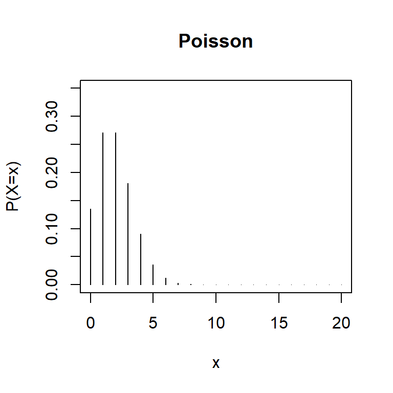

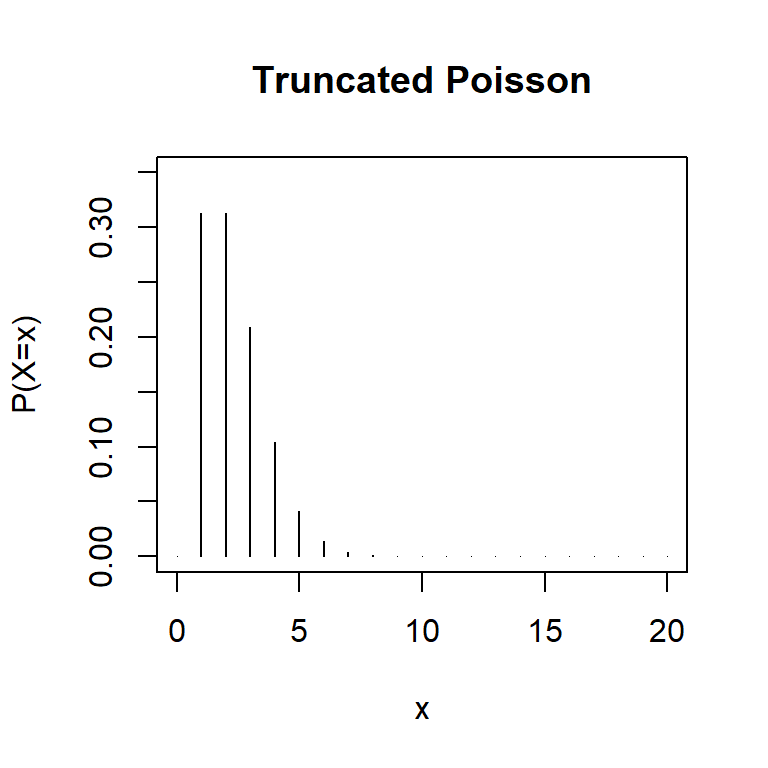
FIGURE 17.3: Comparison of truncated and non-truncated Poisson distributions with \(\lambda = 2\).

It is also straightforward to allow the log mean of the non-zero observations to be modeled as a linear function of predictor variables:

\[\begin{equation} \begin{split} Y_i | Y_i > 0 \sim Poisson(\lambda_i) \\ \log(\lambda_i) = \beta_0 + \beta_1X_{1,i} +\ldots \beta_pX_{p,i} \end{split} \tag{17.2} \end{equation}\]

A few important notes:

• The same (or different) variables may be included in the two model sub-components – i.e., the model for whether or not an observation is 0 (logistic component of the model; (17.1)) and the model for the mean of the non-zero observations (eq. (17.2)).

• \(\lambda_i\) describes the mean of the non-zero observations, not the overall mean of the observations, which is given by: \(E[Y_i|X_i] = (1-p_i)\frac{\lambda_i}{1-e^{-\lambda_i}}\).

For more detail, along with expressions for \(E[Y_i|X_i]\) and \(Var[Y_i|X_i]\) for Poisson and Negative Binomial hurdle models, see page 288 of Zuur et al. (2009).

17.5.2 Hurdle models for continuous response data

The same general approach can be used to model continuous response data with many zeros. For continuous data, the non-zero observations can be modeled using log-normal or gamma distributions. Since these distributions already exclude zeros, there is no need to derive truncated versions of them. Alternatively, it is possible to use a truncated version of continuous probability distributions that allow for negative responses. For example, a truncated Normal distribution could be constructed using \(P(Y | Y>0) = \frac{f(y; \mu, \sigma^2)}{1-F(0; \mu, \sigma^2)}\) where \(F(y) = P(Y \le y)\). We could create a function for calculating the probability density function of a truncated Normal as follows:

dtnorm<-function(x, mean, sd){
    0+I(x>0)*dnorm(x, mean, sd)/(1-pnorm(0, mean, sd))
}

17.6 Zero-inflated mixture models

In the next section, we will model counts of the number of fish that were caught by visitors of a state park. Not everyone that provided data actually fished (and, there is no way of knowing who went fishing and who didn’t since the park did not ask this question of survey respondents). It is easy to imagine two different ways to end up with 0 fish at the end of a camping trip: either you didn’t fish at all or you fished but were not successful. Some predictors may be uniquely suited for modeling whether or not you fished, while others may predict both whether you fished and also how successful you were. Zero-inflated mixture models provide a formal way to model these separate processes.

Like hurdle models, zero-inflated mixture models also have two model sub-components, both of which allow for the possibility of a 0:

1. A model for whether or not an observation is an inflated 0.
2. A count model that also allows for the possibility of a 0.

17.6.1 Marginal distribution

Let’s begin by considering a zero-inflated Poisson model without any covariates. Let \(Y_i\) be our zero-inflated response variable. We can think of \(Y_i\) as being determined by two random processes. First, a coin is flipped to determine if \(Y_i\) is an inflated zero; we get an inflated zero with probability \(\pi\). If \(Y_i\) is not an inflated zero, then we generate a Poisson random number. This allows us to get a 0 in two ways:

• we get an inflated zero with probability \(\pi\)
• we get a non-inflated zero by: 1) not having an inflated zero (occurs with probability \(1- \pi)\), and 2) the Poisson random variable is 0 (occurs with probability \(f(0) =\exp(-\lambda_i)\)). Combining these two probabilities using P(A and B) = P(A)P(B|A), we get the probability of a obtaining a 0 that is not inflated, which is equal to \((1-\pi)e^{-\lambda}\).

To get any non-zero number, we have to: 1) not have an inflated zero (occurs with probability \(1-\pi\)), and 2) the Poisson random variable has to take on the specific value (this occurs with probability \(f(y; \lambda)\)). Thus, the probability that we get a non-zero response, \(y\), is equal to \((1-\pi)f(y; \lambda)\).

Putting all of this together gives us the probability mass function for the zero-inflated Poisson model:

\(P(Y=y) = f(y; \pi, \lambda) =\left\{\begin{array}{ll} \pi + (1-\pi)e^{-\lambda} & \mbox{if } y = 0\\ (1-\pi)\frac{e^{-\lambda}\lambda^y}{y!} & \mbox{if } y = 1, 2, 3, \ldots \end{array} \right.\)

A zero-inflated version of the Negative Binomial can be constructed in much the same way, noting that the probability Mass Function for the Negative Binomial distribution is given by: \(f(y; \mu, \theta) = {y+\theta-1 \choose y}\left(\frac{\theta}{\mu+\theta}\right)^{\theta}\left(\frac{\mu}{\mu+\theta}\right)^y\) and \(f(0; \mu, \theta) = \left(\frac{\theta}{\mu+\theta}\right)^\theta\).

Thus:

\(f(y; \mu, \theta) =\left\{ \begin{array}{ll} \pi + (1-\pi)\left(\frac{\theta}{\mu+\theta}\right)^\theta & \mbox{if } y = 0\\ (1-\pi){y+\theta-1 \choose y}\left(\frac{\theta}{\mu+\theta}\right)^{\theta}\left(\frac{\mu}{\mu+\theta}\right)^y & \mbox{if } y = 1, 2, 3, \ldots \end{array} \right.\)

17.6.2 Zero-inflated mixture models defined using a latent variable

In my description of the zero-inflated mixture model in the previous section, I alluded to two random processes, the first of which was a coin flip to determine whether the response was an inflated 0. The second random process generated a Poisson random number (but only when the first process did not result in an inflated zero). It is often useful to formalize this idea by using a latent or unobserved variable, \(Z_i\), to define the zero-inflation process. Specifically, we may define our zero-inflated Poisson model as:

\[Z_i \sim Bernouli(p_i)\] \[Y_i | Z_i = 0 \sim Poisson(\lambda_i)\]

Alternatively, we may write:

\[Z_i \sim Bernouli(p_i)\] \[Y_i | Z_i \sim Poisson((1-Z_i)\lambda_i)\]

We will use the latter approach to define zero-inflated models in JAGS. In my opinion, this is an area where Bayesian methods shine – they provide an easy way to fit models that can be formulated in terms of latent (unobserved) variables.

As with hurdle models, it is important to understand that \(\lambda_i\) (or \(\mu_i\) if fitting a zero-inflated Negative Binomial) describes the mean, conditional on the observation not being an inflated zero (\(E[Y_i|X_i, Z_i = 0]\)). The unconditional mean and variance are given by⁶⁸:

• \(E[Y_i|X_i] = (1-p_i)\lambda_i\) and \(E[Y_i|X_i] = (1-p_i)\mu_i\) for the Poisson and Negative Binomial distributions, respectively.
  
• \(Var[Y_i|X_i] = (1-p_i)(\lambda_i+p_i\lambda_i^2)\) and \(Var[Y_i|X_i] = (1-p_i)(\mu_i+\frac{\mu_i^2}{\theta})+\mu_i^2p_i(1-p_i)\) for the Poisson and Negative Binomial distributions, respectively.

These expressions are needed when constructing Pearson residuals. As with hurdle models, it is also easy to incorporate predictors that influence the probability of getting an inflated-zero or the mean of our non-inflated observations. Let’s take a look with an applied example.

17.7 Example: Fishing success in state parks

Here, we will consider the zeroinfl function in the pscl package for fitting zero-inflated versions of the Poisson and Negative Binomial models (Jackman, 2020). The zeroinfl function can also be used to fit hurdle models. We will consider a data set and example from UCLA’s Statistical Consulting website. The data have also been incorporated into the Data4Ecologists package and can be accessed using:

data(fish)

The data set is constructed from surveys of 250 groups that visited a state park and contains the following variables:

• count = reported number of fish the group caught
• child = how many children were in the group
• persons = the number of people that were in the group
• camper = 1 if the group brought a camper to the campground and 0 otherwise

On the UCLA page, they considered the following zero-inflated model:

\[\begin{gather} Z_i | X_i \sim Bernoulli(p_i)\\ \text{logit}(p_i) = \gamma_0 + \gamma_1persons_i\\ Y_i|X_i, Z_i \sim Poisson((1-Z_i)\lambda_i)\\ \log(\lambda_i) = \beta_0 + \beta_1 child_i+\beta_2 camper_i \end{gather}\]

I.e., they assumed that the probability of an inflated zero depended on the number of people in the group and that the mean number of fish caught, given the observation was not an inflated zero, depended on the number of children in the group and whether the group brought a camper.

As someone who likes to fish and also camp with family members (3 of whom were once young children), I think a better model would be:

\[\begin{gather} Z_i | X_i \sim Bernoulli(p_i) \\ logit(p_i) = \gamma_0 + \gamma_1child_i \\ Y_i|X_i, Z_i \sim Poisson((1-Z_i)\lambda_i) \\ \log(\lambda_i) = \beta_0 + \beta_1 child_i+\beta_2 camper_i + \beta_3 person_i \end{gather}\]

We can fit this model as follows:

m.zip <- zeroinfl(count ~ child + camper +persons | child, data = fish, dist="poisson")
summary(m.zip)

## 
## Call:
## zeroinfl(formula = count ~ child + camper + persons | child, data = fish, 
##     dist = "poisson")
## 
## Pearson residuals:
##     Min      1Q  Median      3Q     Max 
## -1.4052 -0.7178 -0.4505 -0.1199 26.9595 
## 
## Count model coefficients (poisson with log link):
##             Estimate Std. Error z value Pr(>|z|)    
## (Intercept) -1.05721    0.18123  -5.834 5.42e-09 ***
## child       -1.16755    0.09471 -12.327  < 2e-16 ***
## camper       0.77091    0.09384   8.215  < 2e-16 ***
## persons      0.88856    0.04663  19.056  < 2e-16 ***
## 
## Zero-inflation model coefficients (binomial with logit link):
##             Estimate Std. Error z value Pr(>|z|)    
## (Intercept)  -0.9150     0.2503  -3.655 0.000257 ***
## child         1.1857     0.2654   4.468 7.89e-06 ***
## ---
## Signif. codes:  0 '***' 0.001 '**' 0.01 '*' 0.05 '.' 0.1 ' ' 1 
## 
## Number of iterations in BFGS optimization: 11 
## Log-likelihood:  -766 on 6 Df

The variables on the right hand side of the “|” specify the variables that influence the probability of an inflated zero (in this case, child). We can interpret the coefficients of the zero-inflation part of the model in the same way as we did for logistic regression. We see that the odds of an inflated zero increases by a factor of exp(1.1857) = 3.27 for each additional child in the group. Furthermore, a group with 3 children is exp(1.1857*3) = 35 times more likely to be an inflated zero than a group with 0 children. Lastly, the probability that a group with 3 children is an inflated zero is given by \(\frac{\exp(-0.9150+3 \times 1.1858)}{1+\exp(-0.9150+3 \times 1.1858)}\) and can be calculated using the plogis function:

plogis(-0.9150+3*1.1857)

## [1] 0.9335224

I am not too surprised – it is a lot of work to take 3 children fishing (even if it is incredibly rewarding)! Looking at the count part of the model, we see that groups with children catch fewer fish, whereas larger groups and groups that have a camper tend to catch more fish. Perhaps those with a camper also have better equipment (depth finders, a nice boat, etc). As with standard count models, we can estimate multiplicative effects on the mean number of fish caught, given the observation is not an inflated zero, by exponentiating these parameters. For example, for non-inflated observations, groups with a camper are expected to catch exp(0.77091) = 2.16 times as many fish as groups without a camper.

We can also fit a zero-inflated negative binomial model by changing the distribution argument (dist):

\[\begin{gather} Z_i |X_i \sim Bernoulli(p_i) \\ logit(p_i) = \gamma_0 + \gamma_1child_i \\ Y_i|X_i, Z_i \sim Negative Binomial((1-Z_i)\mu_i, \theta) \\ \log(\mu_i) = \beta_0 + \beta_1 child_i+\beta_2 camper_i + \beta_3 person_i \end{gather}\]

m.zinb <- zeroinfl(count ~ child + camper +persons | child,
               data = fish, dist = "negbin")
summary(m.zinb)

## 
## Call:
## zeroinfl(formula = count ~ child + camper + persons | child, data = fish, 
##     dist = "negbin")
## 
## Pearson residuals:
##      Min       1Q   Median       3Q      Max 
## -0.71609 -0.54836 -0.34329 -0.02088 15.00807 
## 
## Count model coefficients (negbin with log link):
##             Estimate Std. Error z value Pr(>|z|)    
## (Intercept)  -1.6600     0.3197  -5.192 2.08e-07 ***
## child        -1.2056     0.2715  -4.441 8.95e-06 ***
## camper        0.5834     0.2379   2.452   0.0142 *  
## persons       1.0516     0.1110   9.477  < 2e-16 ***
## Log(theta)   -0.5824     0.1823  -3.194   0.0014 ** 
## 
## Zero-inflation model coefficients (binomial with logit link):
##             Estimate Std. Error z value Pr(>|z|)    
## (Intercept)  -4.4302     1.5159  -2.923 0.003472 ** 
## child         2.9263     0.8478   3.452 0.000557 ***
## ---
## Signif. codes:  0 '***' 0.001 '**' 0.01 '*' 0.05 '.' 0.1 ' ' 1 
## 
## Theta = 0.5586 
## Number of iterations in BFGS optimization: 26 
## Log-likelihood: -399.9 on 7 Df

Note that the zeroinfl function parameterizes the overdispersion parameter, \(\theta\) on the log-scale. This ensures that the estimate of \(\theta\), is positive (exp(Log(theta)) = exp(-0.5823) = 0.5586, which is also printed at the bottom of the summary output). The qualitative conclusions are similar to those of the zero-inflated Poisson model, but the coefficients and p-values have changed slightly.

We can compare the two zero-inflated models and also poisson and negative binomial models using AIC (below):

m.pois<- glm(count ~ child + camper + persons, family = poisson, data = fish)
m.nb <- glm.nb(count ~ child + camper + persons, data = fish)
AIC(m.pois, m.nb, m.zip, m.zinb)

##        df       AIC
## m.pois  4 1682.1450
## m.nb    5  820.4440
## m.zip   6 1544.0557
## m.zinb  7  813.8197

This comparison suggests that the zero-inflated negative binomial model provides the best fit to the data, with the non-zero inflated negative binomial model not far behind. The Poisson and zero-inflated Poisson models, by comparison, provide poor fits to the data. My experience, and that of others, is that a Negative Binomial model (without zero-inflation) often “wins” followed by the zero-inflated negative binomial distribution (see e.g., Gray, 2005; Warton, 2005; Sileshi, 2008 for comparative studies).

Lastly, we exponentiate the parameters in our models to summarize effect sizes using incidence ratios for our count models (Table 17.1) and incidence and odds ratios for our zero-inflated models (Table 17.2).

TABLE 17.1: Incidence Ratios [95\(\%\) confidence Intervals]

	Poisson		Negative Binomial
Predictors	Incidence Rate Ratios	CI	Incidence Rate Ratios	CI
(Intercept)	0.14	0.10 – 0.18	0.20	0.10 – 0.38
child	0.18	0.16 – 0.22	0.17	0.11 – 0.24
camper	2.54	2.14 – 3.03	1.86	1.17 – 2.95
persons	2.98	2.76 – 3.22	2.89	2.31 – 3.66
AIC	1682.145		820.444

TABLE 17.2: Odds and Incidence Ratios [95\(\%\) confidence Intervals]

	Zero-Inflated Poisson		Zero-Inflated Negative Binomial
Predictors	Incidence Rate Ratios	CI	Incidence Rate Ratios	CI
(Intercept)	0.35	0.24 – 0.50	0.19	0.10 – 0.36
child	0.31	0.26 – 0.37	0.30	0.18 – 0.51
camper	2.16	1.80 – 2.60	1.79	1.12 – 2.86
persons	2.43	2.22 – 2.66	2.86	2.30 – 3.56
Zero-Inflated Model
(Intercept)	0.40	0.25 – 0.65	0.01	0.00 – 0.23
child	3.27	1.95 – 5.51	18.66	3.54 – 98.29
AIC	1544.056		813.820

17.8 Goodness-of-fit

The AIC comparisons only tell us which of our models is “best”, but they do not tell us if any of the models are actually any good. We could modify our goodness-of-fit test based on Pearson residuals. This would require generating Bernoulli random variables for the zero-inflation process and either Poisson or Negative Binomial random variables for the non-inflated zero observations. We demonstrate this approach when fitting the zero-inflated negative binomial model in JAGS (see Section 17.9). We can also explore plots of the observed counts or Pearson residuals versus fitted values (Figure 17.4).

fish$predict.m.zinb<-predict(m.zinb, type="response")
fish$presiduals.m.zinb<-resid(m.zinb, type="pearson")
p1<-ggplot(fish, aes(predict.m.zinb, count))+geom_point()+
    geom_jitter()+geom_abline(intercept=0,slope=1)+
  xlab("Predicted")+ylab("Observed")

p2<-ggplot(fish, aes(predict.m.zinb, presiduals.m.zinb)) + 
    geom_point() +
    geom_jitter()+
    geom_abline(intercept=0,slope=0) +
    geom_smooth() + 
  xlab("Predicted")+ylab("Pearson Residual")
p1+p2

## `geom_smooth()` using method = 'loess' and formula = 'y ~ x'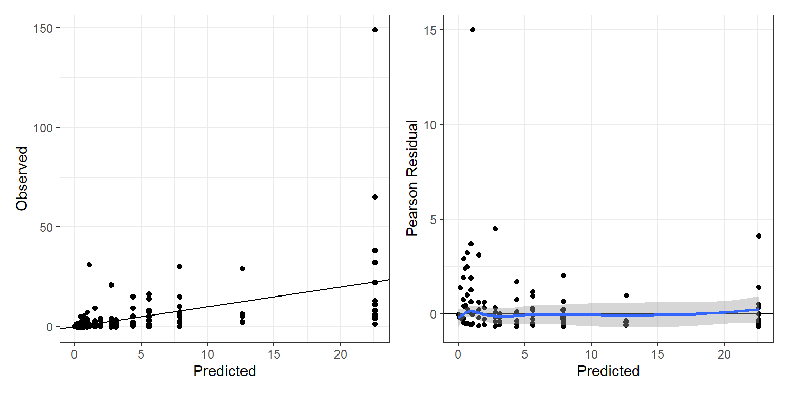

FIGURE 17.4: Observed counts (left panel) and Pearson residuals (right panel) plotted versus fitted values from the zero-inflated Negative Binomial model.

Inspecting these on these two plots (Figure 17.4), there are 2 observations we might want to look into further:

• the group that reported catching ~150 fish (is that even possible?)
• the observation with the large Pearson residual (\(\sim 15\)).

We can use the which.max function to identify these observations:

ind1<-which.max(fish$count) # Max count
ind2<-which.max(fish$presiduals.m.zinb) # Max Pearson residual
fish[c(ind1, ind2),] 

##     count livebait camper persons child predict.m.zinb presiduals.m.zinb
## 89    149        1      1       4     0      22.605575          4.091239
## 138    31        1      0       3     1       1.092746         15.008067

The group that caught 149 fish had 4 people with no children. The observation with the large Pearson residual was for a group of 3 people, one of which was a child, that caught 31 fish. Based on the Pearson residual, we might conclude that the latter observation is actually more of an outlier!

17.9 Bayesian implementation

Here, we follow the approach taken by Kéry (2010). Note that Kery parameterizes the model in terms of \(\psi = 1- \pi\) = the probability of a non zero-inflated response. In comparison to the formulation using zerolinfl, we have:

Parameterization used by zeroinfl:

\(P(Y=y) = f(y) =\left\{\begin{array}{ll} \pi + (1-\pi)e^{-\lambda} & \mbox{if } y = 0\\ (1-\pi)\frac{e^{-\lambda}\lambda^y}{y!} & \mbox{if } y = 1, 2, 3, \ldots \end{array} \right.\)

ZIP model (Kery):

\(P(Y=y) = f(y) =\left\{\begin{array}{ll} 1-\psi + \psi e^{-\lambda} & \mbox{if } y = 0\\ \psi\frac{e^{-\lambda}\lambda^y}{y!} & \mbox{if } y = 1, 2, 3, \ldots \end{array} \right.\)

And, for the Negative Binomial model:

zeroninfl parameterization:

\(f(y) =\left\{ \begin{array}{ll} \pi + (1-\pi)\left(\frac{\theta}{\mu+\theta}\right)^\theta & \mbox{if } y = 0\\ (1-\pi){y+\theta-1 \choose y}\left(\frac{\theta}{\mu+\theta}\right)^{\theta}\left(\frac{\mu}{\mu+\theta}\right)^y & \mbox{if } y = 1, 2, 3, \ldots \end{array} \right.\)

ZINB model (Kery):

\(f(y) =\left\{ \begin{array}{ll} 1-\pi + \pi\left(\frac{\theta}{\mu+\theta}\right)^\theta & \mbox{if } y = 0\\ \pi{y+\theta-1 \choose y}\left(\frac{\theta}{\mu+\theta}\right)^{\theta}\left(\frac{\mu}{\mu+\theta}\right)^y & \mbox{if } y = 1, 2, 3, \ldots \end{array} \right.\)

The only difference is that the coefficients in the logistic part of the model will be of the opposite sign since we are now modeling the probability of a non-inflated zero rather than the probability of an inflated zero.

We use the latent variable approach to implement the Bayesian zero-inflated Negative Binomial model. Specifically, we will create a (partially) latent variable, I.fish (rather than \(Z_i\)), to indicate whether an observation is NOT an inflated 0. We will think of I.fish as an indicator of whether or not the group went fishing (if so, we do not have an inflated 0). We then model count as a Negative Binomial random variable with mean = I.fish\(\times\mu_i\):

\[I.fish_i \sim Bernouli(p_i)\] \[logit(p_i) = \gamma_0 +\gamma_1 child_i\] \[count_i | I.fish_i \sim \mbox{Negative Binomial}(I.fish_i \times \mu_i, \theta)\] \[\log(\mu_i) = \beta_0 + \beta_1 child_i+\beta_2 camper_i + \beta_3 person_i\]

What makes this model different from others that we have considered so far is that we do not actually have a variable in our data set called I.fish that takes on a value of 1 when the group went fishing and 0 otherwise. We will create the I.fish variable, initially setting all of its values to NA (missing). We then set I.fish = 1 for all groups that caught a fish (these cannot be inflated zeros), leaving the value of I.fish = NA for all other observations. JAGS will impute values for I.fish for the observations with missing values during each MCMC iteration using information from the predictor variables for those individuals.

I.fish<-rep(NA, nrow(fish))
I.fish[fish$count>0]<-1 # these people caught fish and are NOT inflated zeros

Think-Pair-Share: How many priors will we need for this model?

znb<-function(){
  
# Priors for count model
 for(i in 1:4){
   beta.c[i] ~ dnorm(0,0.001)
 }
 
# Priors for zero-inflation model (fit on a logit scale)
 for(i in 1:2){
   beta.zi[i] ~ dnorm(0,1/3)
 } 
  
# Overdispersion parameter
  theta ~ dunif(0,50)
    
# Likelihood
  for(i in 1:n){
  # zero-inflation part (logit prob NOT inflated 0, i.e., "went fishing"))  
    logitpsi[i] <- beta.zi[1] + beta.zi[2]*child[i] 
    psi[i] <- exp(logitpsi[i])/(1+exp(logitpsi[i])) # prob Not inflated 0
    I.fish[i] ~ dbern(psi[i]) # Not zero-inflated (i.e., "went fishing") 
     
  # Count part
    log.mu[i] <- beta.c[1] + beta.c[2]*child[i] + beta.c[3]*camper[i] + beta.c[4]*persons[i]
    mu[i] <- exp(log.mu[i])
    mu.eff[i] <- mu[i]*I.fish[i]
    p[i] <- theta/(theta+mu.eff[i])
    count[i] ~ dnegbin(p[i], theta)
  
  # Mean and variances of the observations
  # Derived using:  Var(Count) = E[var(count|z)] + Var[E(count|z)]
    Ey[i] <- mu[i]*psi[i]  
    Vary[i] <- psi[i]*(mu[i] + mu[i]^2/theta) + mu[i]^2*(psi[i]*(1 - psi[i]))
  
  # Generate "new" data
    I.fish.new[i] ~ dbin(psi[i],1)
    mu.eff.new[i] <- mu[i]*I.fish.new[i]
    p.new[i] <- theta/(theta + mu.eff.new[i])
    count.new[i] ~ dnegbin(p.new[i], theta)
  
  # Pearson residuals
    presi[i] <- (count[i] - Ey[i])/sqrt(Vary[i]) # Pearson Resid
    presi.new[i] <- (count.new[i] - Ey[i])/sqrt(Vary[i])

  # Discrepancy measures
    D[i] <- pow(presi[i], 2)
    D.new[i] <- pow(presi.new[i],2)
  }
  fit <- sum(D[])
  fit.new <- sum(D.new[])
}

# Bundle data
jagsdata <- list(count=fish$count, 
                 child=fish$child, 
                 camper = as.numeric(fish$camper) -1, 
                 persons = fish$persons, 
                 n = nrow(fish), 
                 I.fish = I.fish )
                 
# Parameters to estimate
params <- c("beta.zi", "beta.c", "Ey", "psi", "mu", "presi",
            "presi.new", "fit", "fit.new", "theta", "I.fish")


# Start sampler 
out.znb <- jags.parallel(data = jagsdata, parameters.to.save = params, 
                model.file = znb, n.thin = 10, n.chains = 3, n.burnin = 4000, 
                n.iter= 15000)
MCMCsummary(out.znb, params = c("beta.zi", "beta.c", "theta"))

##                  mean        sd        2.5%        50%      97.5% Rhat n.eff
## beta.zi[1]  3.1979630 0.7343385  1.94629281  3.1324735  4.8302946 1.00   957
## beta.zi[2] -2.0270388 0.7593942 -3.16899035 -2.0911349 -0.2854357 1.06   427
## beta.c[1]  -1.0133695 0.3047952 -1.58937586 -1.0101328 -0.4157184 1.00  1387
## beta.c[2]  -1.2259605 0.2949835 -1.82877307 -1.2086964 -0.6647536 1.01  1253
## beta.c[3]   0.5735719 0.2424826  0.08064972  0.5742974  1.0443988 1.00  3300
## beta.c[4]   1.0475373 0.1112952  0.83646516  1.0471353  1.2684389 1.00  1482
## theta       0.5999159 0.1113954  0.41015527  0.5894695  0.8417613 1.01  2147

As always, we should explore traceplots and density plots to make sure that our sampler has converged (Figures 17.5, 17.6).

  denplot(out.znb, parms=c("beta.zi", "beta.c", "theta"), ask=FALSE)

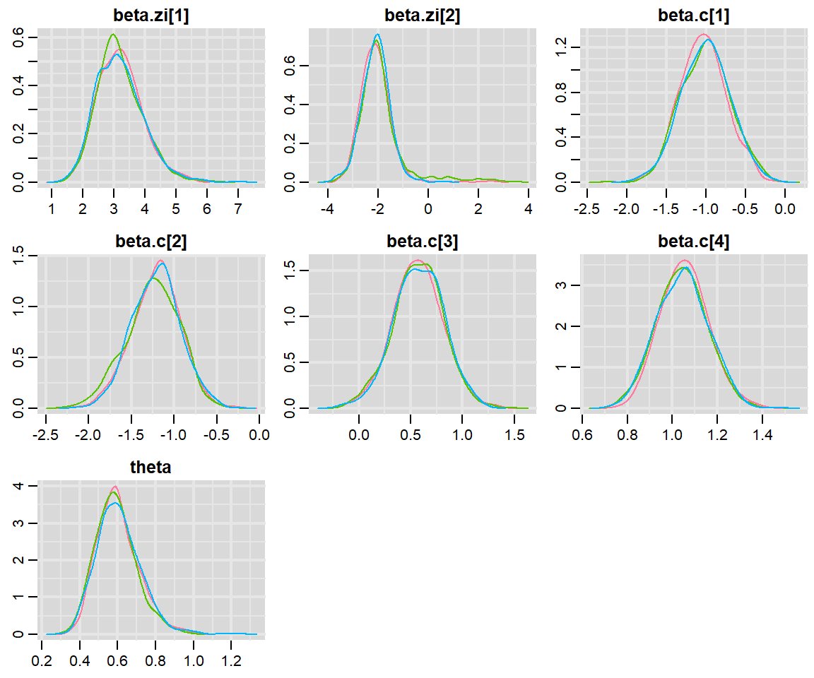
FIGURE 17.5: Posterior density plots from the Bayesian zero-inflated model fit to the fishing data set.

  traplot(out.znb, parms=c("beta.zi", "beta.c", "theta"), ask=FALSE)

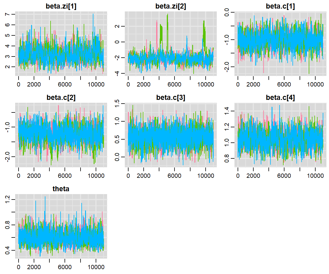
FIGURE 17.6: Trace plots from the Bayesian zero-inflated model fit to the fishing data set.

We can also calculate the Bayesian p-value for the goodness-of-fit test. Although the p-value is fairly small, the conclusions depend critically on the one outlier noted previously with Pearson residual ~ 15. If we drop that observation, the p-value increases substantially (results not shown).

fitstats <- MCMCpstr(out.znb, params = c("fit", "fit.new"), type = "chains") 
T.extreme <- fitstats$fit.new >= fitstats$fit
(p.val <- mean(T.extreme))  

## [1] 0.06181818

Lastly, it may be interesting to look at the imputed values for I.Fish and how they relate to the number of children in each group. Below, we plot the distribution of posterior means for I.fish at each level of child.

fish$I.fish.hat<-out.znb$BUGSoutput$mean$I.fish
ggplot(fish, aes(x = as.factor(child), y = I.fish.hat)) +
    geom_boxplot() + 
    xlab("Number of Children")+ylab("Went fishing?") +
    geom_jitter(color = "black", size = 1, alpha = 0.9)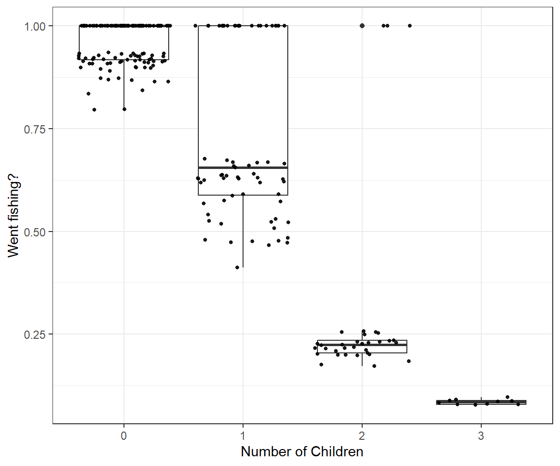

FIGURE 17.7: Boxplots depicting posterior means of I.fish, an indicator that the observation is not an inflated zero, as a function of child.

We see that I.fish is rarely = 1 in groups with 2 or 3 children. This makes sense in light of the fact that no group with 3 children actually caught any fish and the mean number of fish caught for groups with 2 children was less than 1 fish!

fish %>% group_by(child) %>% dplyr::summarize(meanfish=mean(count))

## # A tibble: 4 × 2
##   child meanfish
##   <int>    <dbl>
## 1     0    5.19 
## 2     1    1.76 
## 3     2    0.212
## 4     3    0

17.10 Implementation using glmmTMB

Although the zeroinfl function in the pscl package is probably the most widely used function for fitting zero-inflation models, it is also possible to fit zero-inflated Poisson and zero-inflated negative binomial models using the glmmTMB function in the glmmTMB package (Brooks et al., 2017). The main advantage to using glmmTMB is that it makes it possible to include random effects (e.g., when dealing with non-independent data; see Chapter 18). The glmmTMB function has a separate argument, ziformula, for specifying the zero-inflation part of the model. It also uses the argument family to specify the distribution (either poisson or nbinom2). Below, we demonstrate the equivalence of zero-inflated Poisson models fit using glmmTMB and zeroinfl.

# Equivalent zero-inflated Poisson models
library(glmmTMB)
m.zip.TMB <- glmmTMB(count ~ child + camper + persons, ziformula = ~ child, 
                     data = fish, family  = poisson)
m.zip

## 
## Call:
## zeroinfl(formula = count ~ child + camper + persons | child, data = fish, 
##     dist = "poisson")
## 
## Count model coefficients (poisson with log link):
## (Intercept)        child       camper      persons  
##     -1.0572      -1.1675       0.7709       0.8886  
## 
## Zero-inflation model coefficients (binomial with logit link):
## (Intercept)        child  
##      -0.915        1.186

m.zip.TMB

## Formula:          count ~ child + camper + persons
## Zero inflation:         ~child
## Data: fish
##       AIC       BIC    logLik  df.resid 
## 1544.0557 1565.1845 -766.0279       244 
## 
## Number of obs: 250
## 
## Fixed Effects:
## 
## Conditional model:
## (Intercept)        child       camper      persons  
##     -1.0572      -1.1675       0.7709       0.8886  
## 
## Zero-inflation model:
## (Intercept)        child  
##      -0.915        1.186

And, here, the equivalence between zero-inflated Negative Binomial models fit using glmmTMB and zeroinfl.

# Equivalent zero-inflated Negative Binomial Models
m.zinb.TMB <- glmmTMB(count ~ child + camper + persons, ziformula = ~ child,
                    data = fish, family = nbinom2)
m.zinb

## 
## Call:
## zeroinfl(formula = count ~ child + camper + persons | child, data = fish, 
##     dist = "negbin")
## 
## Count model coefficients (negbin with log link):
## (Intercept)        child       camper      persons  
##     -1.6600      -1.2056       0.5834       1.0516  
## Theta = 0.5586 
## 
## Zero-inflation model coefficients (binomial with logit link):
## (Intercept)        child  
##      -4.430        2.926

m.zinb.TMB

## Formula:          count ~ child + camper + persons
## Zero inflation:         ~child
## Data: fish
##       AIC       BIC    logLik  df.resid 
##  813.8197  838.4700 -399.9099       243 
## 
## Number of obs: 250
## 
## Dispersion parameter for nbinom2 family (): 0.559 
## 
## Fixed Effects:
## 
## Conditional model:
## (Intercept)        child       camper      persons  
##     -1.6600      -1.2056       0.5834       1.0516  
## 
## Zero-inflation model:
## (Intercept)        child  
##      -4.430        2.926

References

Brooks, M. E., Kristensen, K., van Benthem, K. J., Magnusson, A., Berg, C. W., Nielsen, A., … Bolker, B. M. (2017). glmmTMB balances speed and flexibility among packages for zero-inflated generalized linear mixed modeling. The R Journal, 9(2), 378–400. Retrieved from https://journal.r-project.org/archive/2017/RJ-2017-066/index.html

Friederichs, S. J., Zimmer, K. D., Herwig, B. R., Hanson, M. A., & Fieberg, J. (2011). Total phosphorus and piscivore mass as drivers of food web characteristics in shallow lakes. Oikos, 120(5), 756–765.

Gray, B. R. (2005). Selecting a distributional assumption for modelling relative densities of benthic macroinvertebrates. Ecological Modelling, 185(1), 1–12.

Jackman, S. (2020). pscl: Classes and methods for R developed in the political science computational laboratory. Sydney, New South Wales, Australia: United States Studies Centre, University of Sydney. Retrieved from https://github.com/atahk/pscl/

Kéry, M. (2010). Introduction to WinBUGS for ecologists: Bayesian approach to regression, ANOVA, mixed models and related analyses. Academic Press.

Sileshi, G. (2008). The excess-zero problem in soil animal count data and choice of appropriate models for statistical inference. Pedobiologia, 52(1), 1–17.

Warton, D. I. (2005). Many zeros does not mean zero inflation: Comparing the goodness-of-fit of parametric models to multivariate abundance data. Environmetrics: The Official Journal of the International Environmetrics Society, 16(3), 275–289.

Zuur, A., Ieno, E. N., Walker, N., Saveliev, A. A., & Smith, G. M. (2009). Mixed effects models and extensions in ecology with r. Springer Science & Business Media.

---

68. These expressions can be derived fairly easily using \(E[Y]=E_X(E[Y|X])\) and \(Var[Y]=Var_X(E[Y|X]) + E_X(Var[Y|X])\).↩︎