This book is in Open Review. I want your feedback to make the book better for you and other readers. To add your annotation, select some text and then click the on the pop-up menu. To see the annotations of others, click the in the upper right hand corner of the page

Chapter 13 Bayesian linear regression

Learning objectives:

Understand how to fit a linear model using JAGS
Learn how to evaluate goodness-of-fit of models using Bayesian p-values
Be able to calculate credible and prediction intervals for linear models using JAGS

13.1 R packages

We begin by loading a few packages upfront:

library(R2jags) # for interfacing with R
library(MCMCvis) # for summarizing MCMC output
library(mcmcplots) # for plotting MCMC output
library(ggplot2) # for other plots
library(patchwork) # for multi-panel plots
library(dplyr) # for data wrangling

In addition, we will use data and functions from the following packages:

abd (Middleton & Pruim, 2015) to access the LionNoses data set

13.2 Bayesian linear regression

Let’s begin by reconsidering the regression model from Section 1 relating the age of lions to the amount of black pigmentation in their noses:

\[\begin{gather} Age_i \sim N(\mu_i, \sigma^2) \nonumber \\ \mu_i= \beta_0 + \beta_1Proportion.black_i \tag{13.1} \end{gather}\]

Think-pair-share: How many priors will we need to specify when fitting this model?

In this simple model, we have three parameters for which we need to specify priors: $\beta_0, \beta_1$, and $\sigma^2$. You might be temped to also list $\mu_i$, but $\mu_i$ can be derived from $\beta_0, \beta_1$, and our data (i.e., proportion.black), and therefore, we do not need a prior for it. In this book, we will try to specify “non-informative” priors for our parameters – meaning that we do not want our choice of prior to have a large influence on our resulting parameter estimates and their uncertainty. This may not always be simple to do, and in general, it will be wise to:

Give careful consideration to the potential values that the parameters may take on and ensure your prior distribution covers this range of values.
Compare prior and posterior distributions to determine if your prior may have been overly constraining or informative (see Exercise 11.3 here).
Try multiple prior distributions as a form of sensitivity analysis (see Exercise 12.2 here).

Using non-informative priors will allow us to generally arrive at similar conclusions when analyzing data using Bayesian and frequentist methods, which will hopefully allow you to gain confidence in using both approaches. Nonetheless, there are certainly other ways to approach Bayesian modeling. In some situations, you may have additional data that you want to have inform your prior distributions (many Bayesians would certainly advocate for such an approach). Historically, priors were sometimes chosen to “play well” with the likelihood of the data – e.g., to give a closed form solution for the posterior distribution. This leads to choosing a conjugate prior – as we did in our initial example in Section 11.4.3. Priors can also influence the choice of MCMC sampling algorithm and the performance of MCMC samplers. We will not cover these topics here, but they can be of extreme importance, especially when constructing more complex models.

For regression parameters in linear regression models, we will usually use “vague” Normal priors⁵⁷, setting the mean equal to 0 and the precision to a small value (e.g., 0.01 or 0.001, which is equivalent to setting the variance to 100 or 1000). We will generally use uniform $(0, b)$ distributions as a simple and easy way to specify a prior for $\sigma$. As in our “Bayesian t-test” example from Section 12.5, this prior distribution for $\sigma$ will induce a prior distribution for $\tau$, the precision parameter of our Normal distribution.

Below, we specify our JAGS model for the lion data. For now, ignore the code below the likelihood function. We will discuss it when describing a method for performing a goodness-of-fit test for our model (Section 13.4).

# Write model
linreg<-function(){

# Priors
 beta0 ~ dnorm(0,0.001)
 beta1 ~ dnorm(0,0.001)
 sigma ~ dunif(0, 100)

# Derived quantities
 tau <- 1/ (sigma * sigma)

# Likelihood
 for (i in 1:n) {
    age[i] ~ dnorm(mu[i], tau) 
    mu[i] <- beta0 + beta1*proportion.black[i]
 }

# Assess model fit using a sums-of-squares-type discrepancy
 for (i in 1:n) {
    residual[i] <- age[i]-mu[i]       # Residuals for observed data
    sq[i] <- pow(residual[i], 2)    # Squared residuals for observed data

# Generate replicate data and compute fit stats for them
    y.new[i] ~ dnorm(mu[i], tau) # one new data set at each MCMC iteration
    sq.new[i] <- pow(y.new[i]-mu[i], 2)  # Squared residuals for new data
 }
 fit <- sum(sq[])           # Sum of squared residuals for actual data set
 fit.new <- sum(sq.new[])       # Sum of squared residuals for new data set
}

We then bundle our data and call JAGS:

#Load the data
library(abd)
data("LionNoses")

# Bundle data
jags.data <- list(age = LionNoses$age, 
                  proportion.black = LionNoses$proportion.black, 
                  n = nrow(LionNoses))

# Parameters to estimate
params <- c("beta0", "beta1", "sigma", "mu", "y.new", "fit", "fit.new", "residual")

# MCMC settings
nc = 3
ni = 2200
nb = 200
nt = 1

# Start Gibbs sampler
lmbayes <- jags(data = jags.data,  parameters.to.save = params, model.file = linreg, 
n.thin = nt, n.chains = nc, n.burnin = nb, n.iter = ni, progress.bar="none")

## Compiling model graph
##    Resolving undeclared variables
##    Allocating nodes
## Graph information:
##    Observed stochastic nodes: 32
##    Unobserved stochastic nodes: 35
##    Total graph size: 295
## 
## Initializing model

Let’s take a look at the output and compare our results to a frequentist analysis using lm:

lmnoses <- lm(age ~ proportion.black, data = LionNoses)
summary(lmnoses)

## 
## Call:
## lm(formula = age ~ proportion.black, data = LionNoses)
## 
## Residuals:
##     Min      1Q  Median      3Q     Max 
## -2.5449 -1.1117 -0.5285  0.9635  4.3421 
## 
## Coefficients:
##                  Estimate Std. Error t value Pr(>|t|)    
## (Intercept)        0.8790     0.5688   1.545    0.133    
## proportion.black  10.6471     1.5095   7.053 7.68e-08 ***
## ---
## Signif. codes:  0 '***' 0.001 '**' 0.01 '*' 0.05 '.' 0.1 ' ' 1
## 
## Residual standard error: 1.669 on 30 degrees of freedom
## Multiple R-squared:  0.6238, Adjusted R-squared:  0.6113 
## F-statistic: 49.75 on 1 and 30 DF,  p-value: 7.677e-08

MCMCsummary(lmbayes, params = c("beta0", "beta1", "sigma"))

##             mean        sd       2.5%        50%     97.5% Rhat n.eff
## beta0  0.8821171 0.5951552 -0.2817776  0.8795262  2.070602    1  6224
## beta1 10.6459791 1.5965490  7.4334725 10.6659270 13.713155    1  6279
## sigma  1.7399661 0.2377107  1.3493341  1.7172769  2.276687    1  3375

We see that we get similar results using both methods. That should be reassuring.

13.3 Testing assumptions of the model

As we saw in Section 1.5, there are lots of different R packages and functions available for creating residual diagnostic plots for linear regression models. We can build similar plots using the output from JAGS, but it is important to recognize that each residual has its own posterior distribution; we will usually want to summarize these posterior distributions using their mean or median values before creating diagnostic plots.

Think-Pair-Share: Why does each residual have a posterior distribution?

Consider this line of code in our JAGS model:

residual[i] <- age[i]-mu[i]

With each chain, we generated ni = 2200 samples from the posterior distribution of beta0 and beta1. Thus, with each chain, we end up with 2200 samples from the posterior distribution of each mu[i] and 2200 samples from the posterior distribution of each residual[i].

The MCMCpstr function in the MCMCvis package (Youngflesh, 2018) provides a convenient way to access the mean (or other summaries) of the posterior distribution for any parameter. Below, we show how to access the posterior mean of the residuals (residual) and fitted values (mu) so that we can create residual versus fitted value plots, QQ-plots for assessing Normality, and a scale-location plot for evaluating homogeneity of variance (Figure 13.1).

lmresids <- MCMCpstr(lmbayes, params = "residual", func = mean)
lmfitted <- MCMCpstr(lmbayes, params = "mu", func = mean)
jagslmfit <- data.frame(resid = lmresids$residual, fitted = lmfitted$mu)
jagslmfit$std.abs.resid <- sqrt(abs(jagslmfit$resid/sd(jagslmfit$resid)))

And, here we create our plots:

p1 <- ggplot(jagslmfit, aes(fitted, resid)) + geom_point() + 
         geom_hline(yintercept = 0) + geom_smooth()
p2 <- ggplot(jagslmfit, aes(sample = resid)) + stat_qq() + stat_qq_line()
p3 <- ggplot(jagslmfit, aes(fitted, std.abs.resid)) + geom_point() + 
         geom_smooth() + ylab("sqrt(|Standardized Residuals|)")
p1 + p2 + p3

## `geom_smooth()` using method = 'loess' and formula = 'y ~ x'
## `geom_smooth()` using method = 'loess' and formula = 'y ~ x'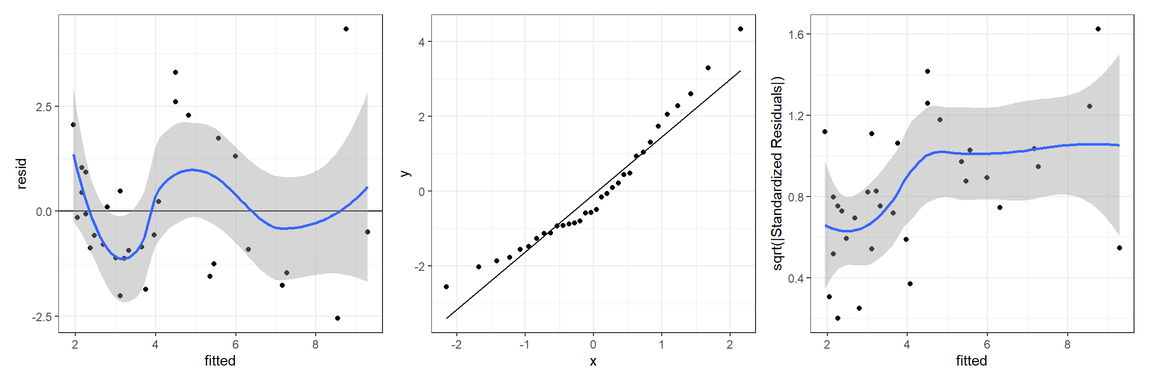

Residual diagnostic plots for a linear model relating the age of lions to the proportion of their nose that is black fit in a Bayesian framework. Plots depict posterior means of the residual and fitted values.

FIGURE 13.1: Residual diagnostic plots for a linear model relating the age of lions to the proportion of their nose that is black fit in a Bayesian framework. Plots depict posterior means of the residual and fitted values.

We can compare Figure 13.1 to similar plots constructed using the output from the frequentist regression using lm (Figure 13.2):

ggResidpanel::resid_panel(lmnoses, plots = c("resid", "qq", "ls"), nrow = 1, smoother = TRUE)

## `geom_smooth()` using formula = 'y ~ x'
## `geom_smooth()` using formula = 'y ~ x'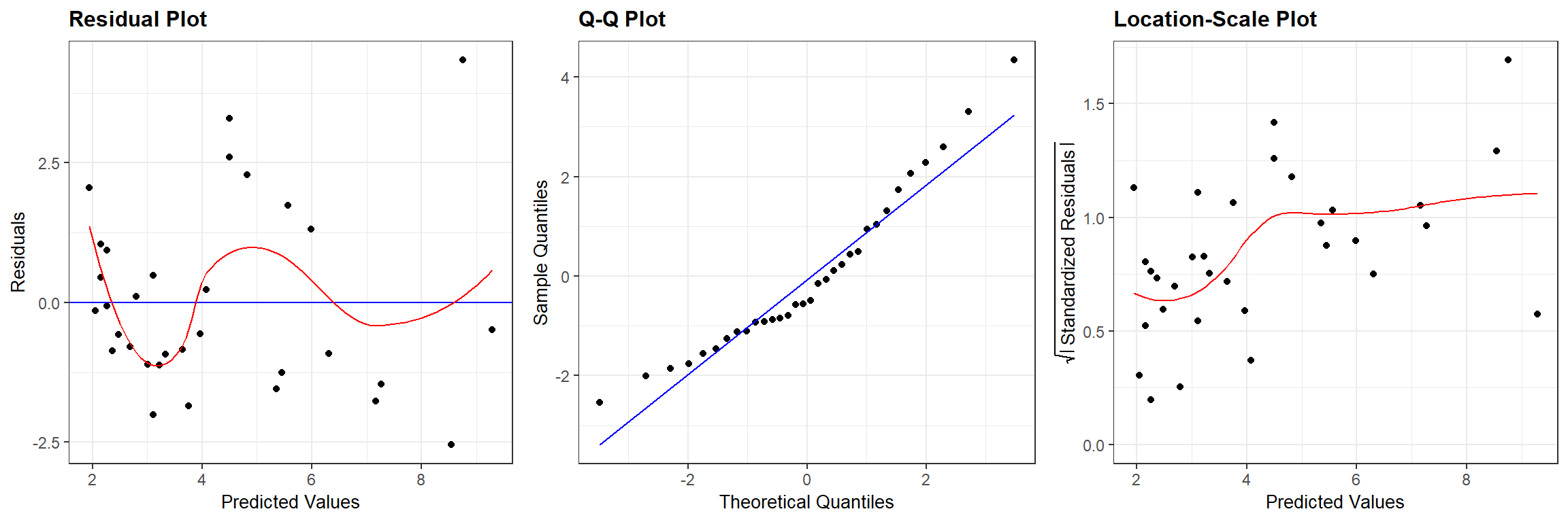

Residual diagnostic plots associated with a linear model relating the age of lions to the proportion of their nose that is black fit in a frequentist framework.

FIGURE 13.2: Residual diagnostic plots associated with a linear model relating the age of lions to the proportion of their nose that is black fit in a frequentist framework.

13.4 Goodness-of-fit testing: Bayesian p-values

In addition to standard residual plots, it is often useful to conduct a formal goodness-of-fit test when evaluating a fitted model. In this section, we will demonstrate a common goodness-of-fit test used to evaluate Bayesian models⁵⁸. Let’s consider the steps involved in any hypothesis test as outlined in Section 1.10.3.

First, we need to state null and alternative hypotheses. As with any goodness-of-fit test, our hypotheses may be stated as:

$H_0:$ the data are consistent with the assumed linear model (eq. (13.1)).

$H_A:$ the data are not consistent with the assumed model.

Next, we need a test statistic, $T$, which will measure the degree to which our data are consistent with the null hypothesis. You are free to choose any test statistic that you want, but ideally the statistic should capture deviations from the null hypothesis that you deem to be important. For example, one might choose to use the number of zeros in a data set as the test statistic when concerned that data may be zero-inflated (Section 17.3). Here, we will use the sum of squared residuals as a general measure of overall fit:

\[T_{obs} = \sum_{i = 1}^n(Y_i - \hat{Y}_i)^2\]

Next, we need to determine the sampling distribution of the test statistic when the null hypothesis is true. We can generate data sets from our assumed model and calculate $T$ for each of these data sets to form this sampling distribution.
Lastly, we compare our test statistic calculated using the observed data, $T_{obs}$, to the sampling distribution of $T$ when when the null hypothesis is true. The p-value is the probability, when the null hypothesis is true, of getting a test statistic, $T_{H_0}$, that is as extreme or more extreme than $T_{obs}$. Ideally, this p-value will be large, suggesting that we do not have much evidence to conclude our assumed model of the data generating process is a poor one.

Now, let’s go back and look at key parts of our specification of the JAGS model, highlighted below:

# Assess model fit using a sums-of-squares-type discrepancy
 for (i in 1:n) {
    residual[i] <- age[i]-mu[i]       # Residuals for observed data
    sq[i] <- pow(residual[i], 2)    # Squared residuals for observed data

# Generate replicate data and compute fit stats for them
    y.new[i] ~ dnorm(mu[i], tau) # one new data set at each MCMC iteration
    sq.new[i] <- pow(y.new[i]-mu[i], 2)  # Squared residuals for new data
 }
 fit <- sum(sq[])           # Sum of squared residuals for actual data set
 fit.new <- sum(sq.new[])       # Sum of squared residuals for new data set

Think-Pair-Share: Which lines of code implement steps 2 and 3 of the hypothesis test?

We calculate $T_{obs}$ using: fit <- sum(sq[]).
We generate new data sets where the null hypothesis is true using: y.new[i] ~ dnorm(mu[i], tau)
We calculate $T_{H_0}$ using: fit.new <- sum(sq.new[])

There is one new wrinkle in all of this, namely that $\hat{Y}_i$ has a posterior distribution, which means that $T_{obs}$ also has a posterior distribution. Nonetheless, we can calculate a Bayesian p-value by comparing the posterior distributions of $T_{obs}$ and $T_{H_0}$. Specifically, we calculate the Bayesian p-value as:

\[\text{p-value} = \sum_{k=1}^M\frac{T_{H_0}^k \ge T_{obs}^k}{M}\] where $k$ indexes the $M$ different posterior samples generated using JAGS. Note, if our model fits poorly, then we should expect that the sums-of-squared residuals associated with our observed data ($T_{obs}$) will be large relative to the sums-of-squared residuals for data generated under the assumed model ($T_{H_0}$). In this case, $T_{H_0}^k$ will rarely be greater than $T_{obs}^k$, we will end up with a small p-value, and we will reject the null hypothesis that the data are consistent with the assumed model. If you get a p-value near 0.5, that is ideal as it suggests that the observed data look very similar to the data generated under the assumed model (at least when it comes to our chosen test statistic). You might wonder at what point (i.e., what threshold for the p-value) should you become concerned about the reliability of your model. I hesitate to give hard and fast rules, but suggest that a p-value less than 0.05 or 0.1 should give you pause⁵⁹.

Below, we calculate this p-value for our linear regression model applied to the LionNoses data set by:

Extracting the MCMC samples using the MCMCpstr function in the MCMCvis package.
Creating an indicator variable that is equal to 1 whenever $T_{H_0}^k \ge T_{obs}^k$ and 0 otherwise.
Calculating the mean of this indicator variable (note, a mean of a 0-1 variable is the same as the proportion of times the variable is equal to 1).

fitstats <- MCMCpstr(lmbayes, params = c("fit", "fit.new"), type = "chains") 
T.extreme <- fitstats$fit.new >= fitstats$fit
(p.val <- mean(T.extreme))

## [1] 0.539

We see that we have a large p-value, suggesting that we do not have strong evidence that our data are inconsistent with the assumed model. That is great news, though we need to keep in mind that our power to detect deviations from the null hypothesis may be low due to our small sample size. In addition, because the data are used twice (once to inform the posterior distribution of our model parameters and then to evaluate fit), these tests tend to produce larger p-values than are generally warranted (see e.g., Conn, Johnson, Williams, Melin, & Hooten, 2018). I.e., we would expect the model to perform more poorly when evaluated against independent data.

Instead of focusing on the numeric p-value, a former student in one of my courses suggested visualizing the posterior distribution of $T_{H_0} -T_{obs}$ (Figure 13.3), which I think is instructive. To create this posterior distribution, we begin by storing the chains in matrix form using the MCMCchains function. We then use the mutate function to create a new variable representing the difference in goodness-of-fit values, with positive values indicating that the model provides a better fit to observed data than the simulated data. We then visualize the p-value (Figure 13.3) using the ShadedDensity function in the WVPlots package (Mount & Zumel, 2021).

#' Posterior for the difference in fits
fitstats <- MCMCchains(lmbayes, params = c("fit", "fit.new")) 
fitstats <- as.data.frame(fitstats) %>% 
  mutate(postdiff = fit.new-fit)
WVPlots::ShadedDensity(frame = fitstats, 
                       xvar = "postdiff",
                       threshold = 0,
                       title = "Posterior distribution: SSE(sim data)-SSE(obs data)",
                       tail = "right")+
  annotate("text", x=85, y = 0.005, 
           label="Better fit to observed data")+
  annotate("text", x=-40, y = 0.005, 
           label="Better fit to simulated data")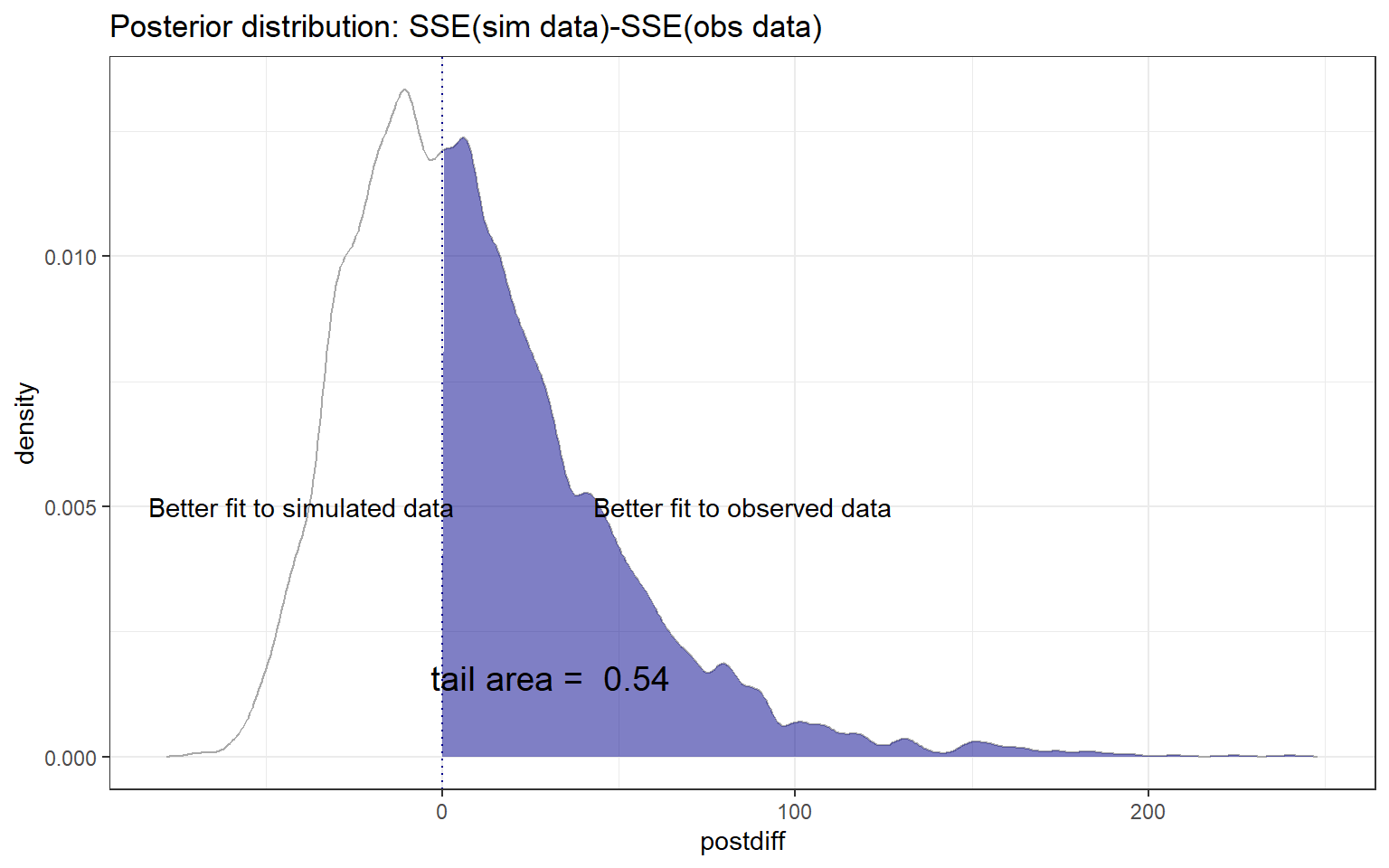

$Posterior distribution of $T_{H_0} -T_{obs}$, where $T_{H_0}$ represents the sum-of-squared residuals for data simulated from the assumed model and $T_{obs}$ represents the sum-of-squared residuals for the observed data. Values greater than 0 indicate a better fit to the observed than simulated data.$

FIGURE 13.3: Posterior distribution of $T_{H_0} -T_{obs}$, where $T_{H_0}$ represents the sum-of-squared residuals for data simulated from the assumed model and $T_{obs}$ represents the sum-of-squared residuals for the observed data. Values greater than 0 indicate a better fit to the observed than simulated data.

The p-value is equal to the area associated with values $>0$, which corresponds to situations where the simulated data have larger sum-of-squared residuals than the observed data.

13.5 Credible intervals

One of the nice things about Bayesian inference is that we can calculate uncertainty for nearly any quantity using posterior distributions of our model parameters. For example, if we want to get predictions of the mean age of lions at a set of values for proportion.black, we can use the posterior distributions for $\beta_0$ and $\beta_1$. Below, we demonstrate how one can accomplish this task using a for loop to get predictions for 10 equally spaced values of proportion.black over the range of the observed data.

First, we pull off and store the MCMC samples of $\beta_0$ and $\beta_1$ using the MCMCpstr function with type = "chains" in the MCMCvis package.

betas <- MCMCpstr(lmbayes, params = c("beta0", "beta1"), type = "chains")

We see that we have a total of 6000 MCMC samples from the posterior distribution of $(\beta_0, \beta_1)$ (i.e., 3 chains x 2000 samples per chain):

dim(betas$beta0)

## [1]    1 6000

Next, we create a vector of values for proportion.black for which we desire predictions:

prop.black <-seq(from = min(LionNoses$proportion.black), 
                 to = max(LionNoses$proportion.black), 
                 length = 10)

We then loop over the 10 different values of prop.black, estimate the mean age using each of our MCMC samples of $\beta_0$ and $\beta_1$, and then find the 2.5 and 97.5 quantiles of the resulting estimates to form our 95% credible interval for each value of prop.black:

# Number of MCMC samples
nmcmc <- dim(betas$beta0)[2]

# Number of unique values of proportion.black where we want predictions
nlions <- length(prop.black)

# Set up a matrix to hold 95% credible intervals for each value of prop.black
conf.int <- matrix(NA, nlions, 2) 

# Loop over values for proportion.black
for(i in 1:nlions){
  # Estimate the mean age for the current value of prop.black and for 
  #   each MCMC sample of beta0 and beta1. Note: rep(prop.black[i], nmcmc)
  #   creates a vector of the current prop.black values that is equal in
  #   length to the vector of betas from the MCMC sampler.
  age.hats <- betas$beta0 + rep(prop.black[i], nmcmc)*betas$beta1
  conf.int[i,] <- quantile(age.hats, prob = c(0.025, 0.975))
}

Next, we combine our credible interval with predictions for each age using the mean of the posterior distribution of $\beta_0$ and $\beta_1$ and plot the results (Figure 13.4).

beta.hat <- MCMCpstr(lmbayes, params = c("beta0", "beta1"), func = mean)
phats <- data.frame(est = rep(beta.hat$beta0, nlions) + rep(beta.hat$beta1, nlions)*prop.black, 
                    LCL = conf.int[,1], 
                    UCL = conf.int[,2], proportion.black = prop.black)
ggplot(phats, aes(proportion.black, est)) +
  geom_ribbon(aes(ymin = LCL, ymax = UCL), fill = "grey70", alpha = 2) +
  geom_line() +ylab("Age") + 
  geom_point(data = LionNoses, aes(proportion.black, age))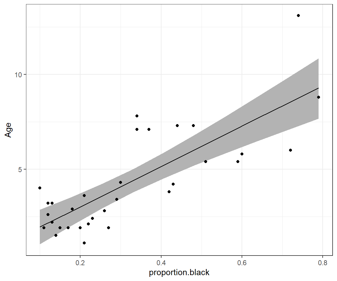

FIGURE 13.4: 95% credible interval for the mean age as a function of proportion.black.

Think-Pair-Share: How could we modify the code in this section to produce a 95% prediction interval?

13.6 Prediction intervals

Recall that prediction intervals need to consider not only the uncertainty associated with the regression line but also the variability of the observations about the line. This variability is modeled using a Normal distribution with standard deviation $\sigma$. This presents a simple way forward - we just need to simulate added variability about the line using rnorm and can use our posterior distribution for $\sigma$ when generating these values.

# Pull off the samples from the posterior distribution of sigma
sigmap <- MCMCpstr(lmbayes, params = "sigma", type = "chains")$sigma

# Set up a matrix to hold 95% prediction intervals for each value of prop.black
pred.int <- matrix(NA, nlions, 2) 

# Loop over values for proportion.black
for(i in 1:nlions){
  # Estimate the mean age for the current value of prop.black and for
  #    each MCMC sample of beta0 and beta1
  age.inds <- betas$beta0 + rep(prop.black[i], nmcmc)*betas$beta1 + 
                     rnorm(nmcmc, mean = 0, sd = sigmap)
  # Now for prediction intervals using the quantiles of the age values
  pred.int[i,] <- quantile(age.inds, prob = c(0.025, 0.975))
}

Now, we can add the prediction intervals to our plot (Figure 13.5).

beta.hat <- MCMCpstr(lmbayes, params = c("beta0", "beta1"), func = mean)
phats <- data.frame(phats, 
                    LPL = pred.int[,1], 
                    UPL = pred.int[,2])
ggplot(phats, aes(proportion.black, est)) +
  geom_line(aes(proportion.black, LCL), col = "red", lty = 2) +
  geom_line(aes(proportion.black, UCL), col = "red", lty = 2) +
  geom_line(aes(proportion.black, LPL), col = "blue", lty = 2) +
  geom_line(aes(proportion.black, UPL), col = "blue", lty = 2) +
  geom_line() +ylab("Age") + 
  geom_point(data = LionNoses, aes(proportion.black, age))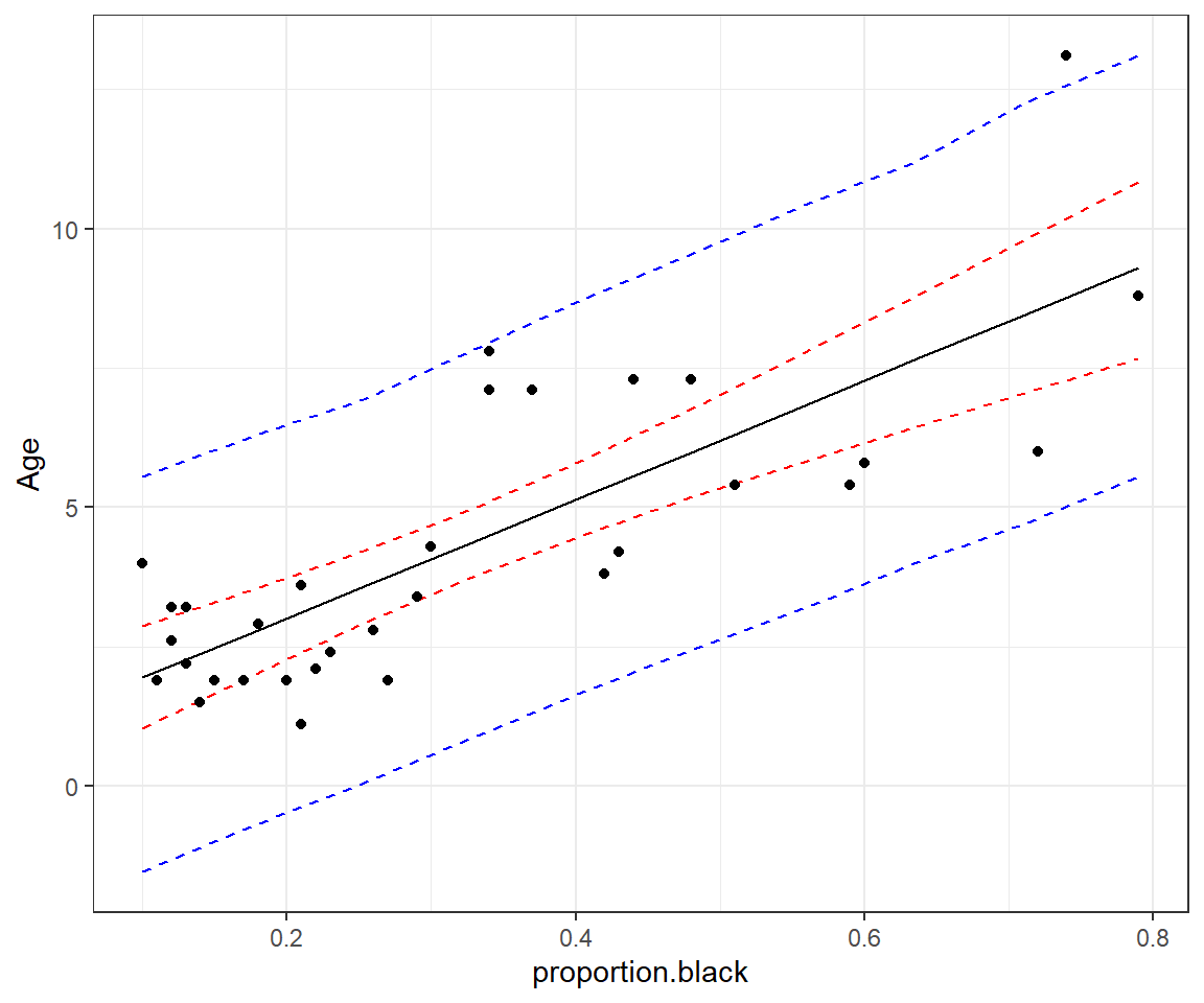

FIGURE 13.5: 95% credible (red) and prediction (blue) intervals for age as a function of proportion.black.

13.7 Credible and prediction intervals the easy way

The above examples are nice in that they demonstrate how you can easily calculate derived quantities using samples from the posterior distributions. However, there is an easier way to get both credible intervals and prediction intervals, and that is, to have JAGS do all the calculations for us and save the necessary output.

If we look at our JAGS code, below, we actually had everything we needed to calculate credible intervals and prediction intervals.

Think-Pair-Share: Can you think of an easier way to calculate credible intervals and prediction intervals from quantities that JAGS is already computing?

linreg<-function(){

# Priors
 beta0 ~ dnorm(0,0.001)
 beta1 ~ dnorm(0,0.001)
 sigma ~ dunif(0, 100)

# Derived quantities
 tau <- 1/ (sigma * sigma)

# Likelihood
 for (i in 1:n) {
    age[i] ~ dnorm(mu[i], tau) 
    mu[i] <- beta0 + beta1*proportion.black[i]
 }

# Assess model fit using a sums-of-squares-type discrepancy
 for (i in 1:n) {
    residual[i] <- age[i]-mu[i]       # Residuals for observed data
    sq[i] <- pow(residual[i], 2)    # Squared residuals for observed data

# Generate replicate data and compute fit stats for them
    y.new[i] ~ dnorm(mu[i], tau) # one new data set at each MCMC iteration
    sq.new[i] <- pow(y.new[i]-mu[i], 2)  # Squared residuals for new data
 }
 fit <- sum(sq[])           # Sum of squared residuals for actual data set
 fit.new <- sum(sq.new[])       # Sum of squared residuals for new data set
}

Note that:

JAGS has already sampled from the posterior distribution of the mean age for the values of proportion.black in our data set – i.e., mu[i]. These can be used to form credible intervals.
JAGS has already generated new observations from our assumed model – i.e., y.new[i]. These can be used to form prediction intervals.

Below, we demonstrate that these outputs could be used to form credible and prediction intervals.

CI <- MCMCpstr(lmbayes, params = c("mu"), 
               func = function(x) quantile(x, probs = c(0.025, 0.975)))$mu
PI <- MCMCpstr(lmbayes, params = c("y.new"), 
               func = function(x) quantile(x, probs = c(0.025, 0.975)))$y.new

Plotting these results (Figure 13.6), we see that we get nearly identical intervals as in Figure 13.5:

phats2 <- data.frame(est =MCMCpstr(lmbayes, params = c("mu"), func = mean)$mu, 
                     proportion.black = LionNoses$proportion.black,
                    LCL = CI[,1], 
                    UCL = CI[,2], 
                    LPL = PI[,1], 
                    UPL = PI[,2])
ggplot(phats2, aes(proportion.black, est)) +
  geom_line(aes(proportion.black, LCL), col = "red", lty = 2) +
  geom_line(aes(proportion.black, UCL), col = "red", lty = 2) +
  geom_line(aes(proportion.black, LPL), col = "blue", lty = 2) +
  geom_line(aes(proportion.black, UPL), col = "blue", lty = 2) +
  geom_line() +ylab("Age") + 
  geom_point(data = LionNoses, aes(proportion.black, age))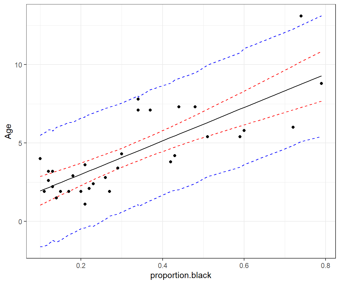

FIGURE 13.6: 95% credible (red) and prediction (blue) intervals for age as a function of proportion.black.

References

Conn, P. B., Johnson, D. S., Williams, P. J., Melin, S. R., & Hooten, M. B. (2018). A guide to bayesian model checking for ecologists. Ecological Monographs, 88(4), 526–542.

Middleton, K. M., & Pruim, R. (2015). Abd: The analysis of biological data. Retrieved from https://CRAN.R-project.org/package=abd

Mount, J., & Zumel, N. (2021). WVPlots: Common plots for analysis. Retrieved from https://CRAN.R-project.org/package=WVPlots

Youngflesh, C. (2018). MCMCvis: Tools to visualize, manipulate, and summarize MCMC output. Journal of Open Source Software, 3(24), 640. doi:10.21105/joss.00640

The meaning of vague here is that the prior distribution allows for a wide range of potential values.↩︎
A similar approach can be implemented for frequentist models as we will see in Section 15.4.5.↩︎
Note that it is possible, though fairly unlikely, that a model will fit the observed data much better than data generated from the assumed model, resulting in a Bayesian p-value that is close to 1. In this case, it is also worth digging a little deeper to see why this may have occurred.↩︎